Difference between revisions of "Batch reactor"
FelixMueller (Talk | contribs) |
(<math> </math> rendering appears to be broken) |
||
| (12 intermediate revisions by 2 users not shown) | |||
| Line 3: | Line 3: | ||
|nx = 2 | |nx = 2 | ||
|nu = 1 | |nu = 1 | ||
| + | |nc = 2 | ||
|nre = 2 | |nre = 2 | ||
}} | }} | ||
| Line 17: | Line 18: | ||
<p> | <p> | ||
<math> | <math> | ||
| − | \begin{array}{ | + | \begin{array}{llcl} |
\displaystyle \max_{x, u} & x_2(t_f) \\[1.5ex] | \displaystyle \max_{x, u} & x_2(t_f) \\[1.5ex] | ||
| − | \mbox{s.t.} & \dot{x}_1 | + | \mbox{s.t.} & \dot{x}_1 & = & -k_1 x_1^2.\\ |
| − | & \dot{x}_2 | + | & \dot{x}_2 & = & k_1 x_1^2 - k_2 x_2,\\ |
| − | & k_1 & = & 4000 \; e^{(-2500/T(t))} | + | & k_1 & = & 4000 \; e^{(-2500/T(t))}, \\ |
| − | & k_2 & = & 620000 \; e^{(-5000/T(t))} | + | & k_2 & = & 620000 \; e^{(-5000/T(t))}, \\[1.5ex] |
& x(0) &=& (1, 0)^T, \\ | & x(0) &=& (1, 0)^T, \\ | ||
| − | & T(t) &\in& [298, 398 | + | & T(t) &\in& [298, 398]. |
\end{array} | \end{array} | ||
</math> | </math> | ||
</p> | </p> | ||
| − | <math> x_1(t) </math> and <math> x_2(t) </math> | + | <math> x_1(t) </math> and <math> x_2(t) </math> represent the concentrations of A and B at timepoint <math> t </math> respectively. The control function <math> T(t) </math> represents the temperature. |
== Parameters == | == Parameters == | ||
| Line 39: | Line 40: | ||
This solution was computed using JuMP with a collocation method and 300 discretization points. The differential equations were solved using the explicit Euler Method. The source code can be found at [[Batch reactor (JuMP)]]. | This solution was computed using JuMP with a collocation method and 300 discretization points. The differential equations were solved using the explicit Euler Method. The source code can be found at [[Batch reactor (JuMP)]]. | ||
| − | The optimal objective value of the problem is | + | The optimal objective value of the problem is x2(tf) = 0.611715. |
<gallery caption="Reference solution plots" widths="180px" heights="140px" perrow="2"> | <gallery caption="Reference solution plots" widths="180px" heights="140px" perrow="2"> | ||
| Line 49: | Line 50: | ||
Model descriptions are available in | Model descriptions are available in | ||
| + | * [[:Category:Gekko | GEKKO Python code]] at [[Batch reactor (GEKKO)]] | ||
* [[:Category: Julia/JuMP | JuMP code]] at [[Batch reactor (JuMP)]] | * [[:Category: Julia/JuMP | JuMP code]] at [[Batch reactor (JuMP)]] | ||
| Line 57: | Line 59: | ||
[[Category:MIOCP]] | [[Category:MIOCP]] | ||
[[Category:ODE model]] | [[Category:ODE model]] | ||
| + | [[Category:Chemical engineering]] | ||
Latest revision as of 14:42, 11 April 2019
| Batch reactor | |
|---|---|
| State dimension: | 1 |
| Differential states: | 2 |
| Continuous control functions: | 1 |
| Path constraints: | 2 |
| Interior point equalities: | 2 |
This batch reactor problem describes the consecutive reaction of some substance A via substance B into a desired product C.
The system is interacted with via the control function  which stands for the temperature.
The goal is to produce as much of substance B (which can then be converted into product C) as possible within the time limit.
Mathematical formulation
The optimal control problem is given by
![\begin{array}{llcl}
\displaystyle \max_{x, u} & x_2(t_f) \\[1.5ex]
\mbox{s.t.} & \dot{x}_1 & = & -k_1 x_1^2.\\
& \dot{x}_2 & = & k_1 x_1^2 - k_2 x_2,\\
& k_1 & = & 4000 \; e^{(-2500/T(t))}, \\
& k_2 & = & 620000 \; e^{(-5000/T(t))}, \\[1.5ex]
& x(0) &=& (1, 0)^T, \\
& T(t) &\in& [298, 398].
\end{array}](https://mintoc.de/images/math/9/f/7/9f71534dc1a851a90b41b50d9ab369a9.png)
 and
and  represent the concentrations of A and B at timepoint
  respectively. The control function
  represents the temperature.
Parameters
The starting time and end time are given by ![[t_0, t_f] = [0, 1]](https://mintoc.de/images/math/9/0/d/90d354576ba03d7a9fb1d63ba2ecc7cc.png) .
.
Reference Solutions
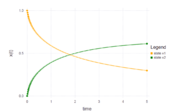
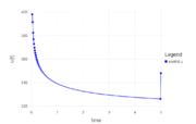
This solution was computed using JuMP with a collocation method and 300 discretization points. The differential equations were solved using the explicit Euler Method. The source code can be found at Batch reactor (JuMP).
The optimal objective value of the problem is x2(tf) = 0.611715.
- Reference solution plots
Source Code
Model descriptions are available in
References
The problem can be found in the Tomlab PROPT guide or in the Dynopt guide.


 .
.