Difference between revisions of "Electric Car"
FelixMueller (Talk | contribs) (→Mathematical formulation) |
FelixMueller (Talk | contribs) |
||
| (12 intermediate revisions by the same user not shown) | |||
| Line 3: | Line 3: | ||
|nx = 4 | |nx = 4 | ||
|nw = 1 | |nw = 1 | ||
| + | |nc = 2 | ||
|nri = 2 | |nri = 2 | ||
|nre = 5 | |nre = 5 | ||
| Line 20: | Line 21: | ||
\displaystyle \min_{x, u} & x_3(t_f) \\[1.5ex] | \displaystyle \min_{x, u} & x_3(t_f) \\[1.5ex] | ||
\mbox{s.t.} | \mbox{s.t.} | ||
| − | & \dot{x}_0 & = & | + | & \dot{x}_0 & = & (V_{alim} u - R_m x_0 - K_m x_1) / L_m, \\ |
| − | + | & \dot{x}_1 & = & \frac{K_r^2}{Mr^2} (K_m x_0 - \frac{r}{K_r} ( M g K_f + \frac{1}{2} \rho S C_x \frac{r^2}{K_r^2} x_1^2)), \\ | |
| − | + | & \dot{x}_2 & = & \frac{r}{K_r} x_1, \\ | |
& \dot{x}_3 & = & V_{alim} u x_0 + R_{bat} x_0^2, \\[1.5ex] | & \dot{x}_3 & = & V_{alim} u x_0 + R_{bat} x_0^2, \\[1.5ex] | ||
| − | + | & x(t_0) &=& (0,0,0,0)^T, \\ | |
& x(t_f) & \in & \mathcal{T} \subseteq \mathbb{R}^4,\\ | & x(t_f) & \in & \mathcal{T} \subseteq \mathbb{R}^4,\\ | ||
& x_0(t) & \in & [-i_{max}, i_{max}], \\ | & x_0(t) & \in & [-i_{max}, i_{max}], \\ | ||
| Line 104: | Line 105: | ||
|- | |- | ||
|Resistance of the battery | |Resistance of the battery | ||
| − | |<math>R_ | + | |<math>R_{bat}</math> |
|0.05 | |0.05 | ||
|<math> Ohms </math> | |<math> Ohms </math> | ||
| Line 111: | Line 112: | ||
== Reference Solutions == | == Reference Solutions == | ||
| − | We look at the particular instance of our problem with <math> t_f = 10s </math>and target set <math> \mathcal{T} | + | We look at the particular instance of our problem with <math> t_f = 10s </math>and target set <math> \mathcal{T} = \mathbb{R} \times \mathbb{R} \times \{100\} \times \mathbb{R} </math>, in which the car needs to cover 100m in 10s. |
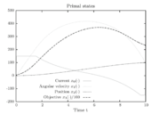
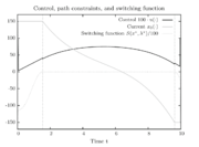
Figure 1 shows a plot of the differential states of the optimal trajectory of the relaxed problem (i.e. <math> u \in [-1,1] </math>instead of <math> u \in \{-1,1\} </math>) for <math> N = 1000, N </math>being the number of time discretization points. The current <math> x_0 </math>increases to its maximal value of 150A, stays there for a certain time, decreases on its minimal value of -150A, stays on this value and eventually increases slightly. This behavior corresponds to the different arcs bang, path-constrained, singular, path-constrained, bang and can be observed also in Figure 2. It shows the corresponding switching function and the optimal control. Note that the plots show data from the solution with the indirect approach. | Figure 1 shows a plot of the differential states of the optimal trajectory of the relaxed problem (i.e. <math> u \in [-1,1] </math>instead of <math> u \in \{-1,1\} </math>) for <math> N = 1000, N </math>being the number of time discretization points. The current <math> x_0 </math>increases to its maximal value of 150A, stays there for a certain time, decreases on its minimal value of -150A, stays on this value and eventually increases slightly. This behavior corresponds to the different arcs bang, path-constrained, singular, path-constrained, bang and can be observed also in Figure 2. It shows the corresponding switching function and the optimal control. Note that the plots show data from the solution with the indirect approach. | ||
| Line 118: | Line 119: | ||
The direct and indirect approaches are local optimization techniques and only provide upper bounds for the relaxed problem and hence for the original problem. Here the indirect solution of the relaxed problem gives us a bound of <math> x_3(t_f) = 22777.2 </math>. | The direct and indirect approaches are local optimization techniques and only provide upper bounds for the relaxed problem and hence for the original problem. Here the indirect solution of the relaxed problem gives us a bound of <math> x_3(t_f) = 22777.2 </math>. | ||
| + | |||
| + | |||
| + | <gallery caption="Reference solution plots" widths="180px" heights="140px" perrow="3"> | ||
| + | Image:ElectricCar PrimalStates Plot.PNG| Primal states of an optimal trajectory for the relaxed problem on a control discretization grid with <math> N = 1,000 </math>. | ||
| + | Image:ElectricCar Control PathConstraints SwitchingFunction Plot.PNG| The optimal control and switching function. The dotted vertical lines show the switching times <math> \tau_i </math> where transitions between different kinds of arcs occur. | ||
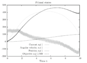
| + | Image:ElectricCar PrimalStates SumUpRounding.PNG| Primal states with Sum up rounding on grid with <math> \Delta t = 10^{-2} </math>. | ||
| + | </gallery> | ||
== Source Code == | == Source Code == | ||
| Line 128: | Line 136: | ||
There are several alternative formulations and variants of the above problem, in particular | There are several alternative formulations and variants of the above problem, in particular | ||
| − | * fixed final velocity, <math> \mathcal{T} = \mathbb{R} \times \{ 50 \frac{K_r}{3.6r} \} \times \{100\} \times \mathbb{R}, | + | * fixed final velocity, <math> \mathcal{T} = \mathbb{R} \times \{ 50 \frac{K_r}{3.6r} \} \times \{100\} \times \mathbb{R}, t_f = 10s </math> |
| − | * bounded velocity, <math> | + | * bounded velocity, <math> \mathcal{T} = \mathbb{R} \times \mathbb{R} \times \{100\} \times \mathbb{R}, t_f = 10s, x_2(t) \leq 45 \frac{K_r}{3.6r} \forall t </math> |
| − | * fixed final velocity, bounded velocity, longer time horizon, <math> x_2(t) \leq 30 \frac{K_r}{3.6r} \forall t, \mathcal{T} = \mathbb{R} \times \{ 30 \frac{K_r}{3.6r} \} \times \{100\} \times \mathbb{R}, | + | * fixed final velocity, bounded velocity, longer time horizon, <math> x_2(t) \leq 30 \frac{K_r}{3.6r} \forall t, \mathcal{T} = \mathbb{R} \times \{ 30 \frac{K_r}{3.6r} \} \times \{100\} \times \mathbb{R}, t_f = 15s </math>. |
== References == | == References == | ||
Latest revision as of 09:29, 27 July 2016
| Electric Car | |
|---|---|
| State dimension: | 1 |
| Differential states: | 4 |
| Discrete control functions: | 1 |
| Path constraints: | 2 |
| Interior point inequalities: | 2 |
| Interior point equalities: | 5 |
The Electric car problem tries to find an optimal driving policy for an electric car. The goal is to use minimal energy to finish a given distance. As the car can be driven in two discrete modes, which either cause acceleration (and thereby consumption of energy) or the recharging of the battery, the control variable  is supposed to be integer. Additionally the model for the electric car itself contains nonlinearities.
The problem is discussed in detail in [Sager2015]Author: Sager, S.; M. Claeys; F. Messine
Journal: Journal of Global Optimization
Number: 4
Pages: 721--743
Title: Efficient upper and lower bounds for global mixed-integer optimal control
Volume: 61
Year: 2015 .
.
Contents
Mathematical formulation
The mixed-integer optimal control problem is given by
![\begin{array}{llclr}
\displaystyle \min_{x, u} & x_3(t_f) \\[1.5ex]
\mbox{s.t.}
& \dot{x}_0 & = & (V_{alim} u - R_m x_0 - K_m x_1) / L_m, \\
& \dot{x}_1 & = & \frac{K_r^2}{Mr^2} (K_m x_0 - \frac{r}{K_r} ( M g K_f + \frac{1}{2} \rho S C_x \frac{r^2}{K_r^2} x_1^2)), \\
& \dot{x}_2 & = & \frac{r}{K_r} x_1, \\
& \dot{x}_3 & = & V_{alim} u x_0 + R_{bat} x_0^2, \\[1.5ex]
& x(t_0) &=& (0,0,0,0)^T, \\
& x(t_f) & \in & \mathcal{T} \subseteq \mathbb{R}^4,\\
& x_0(t) & \in & [-i_{max}, i_{max}], \\
& u(t) &\in& \{-1, 1\}.
\end{array}](https://mintoc.de/images/math/f/8/1/f81a52adee4116324d4656c5e4256abb.png)
Here the four differential states stand for the electrical current ( ), the angular velocity (
 ), the position of the car (
 ), and the consumed energy (
 ). The objective function
  is just a reformulation of the Lagrange-type objective function tracking the used energy over time.
Parameters
These fixed values are used within the model.
| Name | Symbol | Value | Unit |
| Coefficient of reduction | 
|
10 | [-] |
| Air density | 
|
1.293 | 
|
| Aerodynamic coefficient | 
|
0.4 | [-] |
| Area in the front of the vehicle | 
|
2 | 
|
| Radius of the wheel | 
|
0.33 | 
|
| Constant representing the friction of the wheels on the road | 
|
0.03 | [-] |
| Coefficient of the motor torque | 
|
0.27 | [-] |
| Inductor resistance | 
|
0.03 | 
|
| inductance of the rotor | 
|
0.05 | [-] |
| Mass | 
|
250 | 
|
| Gravity constant | 
|
9,81 | [-] |
| Battery voltage | 
|
150 | 
|
| Resistance of the battery | 
|
0.05 | 
|
Reference Solutions
We look at the particular instance of our problem with  and target set
  , in which the car needs to cover 100m in 10s.
Figure 1 shows a plot of the differential states of the optimal trajectory of the relaxed problem (i.e.
 ![u \in [-1,1]](https://mintoc.de/images/math/7/7/e/77ebca4c196d281ab127d484baf6bd92.png) instead of
instead of  ) for
) for  being the number of time discretization points. The current
  increases to its maximal value of 150A, stays there for a certain time, decreases on its minimal value of -150A, stays on this value and eventually increases slightly. This behavior corresponds to the different arcs bang, path-constrained, singular, path-constrained, bang and can be observed also in Figure 2. It shows the corresponding switching function and the optimal control. Note that the plots show data from the solution with the indirect approach.
Applying the sum up rounding strategy results in an integer-feasible chattering solution.
The resulting primal states are shown in Figure 3. One observes the high-frequency zig-zagging of the current  that results from the fast switches in the control.
The direct and indirect approaches are local optimization techniques and only provide upper bounds for the relaxed problem and hence for the original problem. Here the indirect solution of the relaxed problem gives us a bound of  .
.
- Reference solution plots
Source Code
Model descriptions are available in
Variants
There are several alternative formulations and variants of the above problem, in particular
- fixed final velocity,

- bounded velocity,

- fixed final velocity, bounded velocity, longer time horizon,
 .
.
References
| [Sager2015] | Sager, S.; M. Claeys; F. Messine (2015): Efficient upper and lower bounds for global mixed-integer optimal control. Journal of Global Optimization, 61, 721--743 |  |

 .
.

 where transitions between different kinds of arcs occur.

 .
.