SEIR Epidemic

SEIR Epidemic
State dimension:	1
Differential states:	4
Discrete control functions:	2

The SEIR epidemic optimal control problem models the spread of an infectious disease through a homogeneous population divided into four compartments: susceptible ($S$), exposed ($E$), infectious ($I$), and recovered ($R$). Two controls are applied simultaneously: a vaccination rate that removes susceptible individuals from the transmission chain, and a social-distancing intensity that reduces the effective contact rate. The objective is to minimise a weighted combination of the cumulative infectious burden and the quadratic costs of both interventions over a finite horizon, yielding a trade-off between disease suppression and resource expenditure. The problem is nonlinear and non-convex and is calibrated to a COVID-19-like baseline scenario.

Mathematical formulation

$\begin{array}{lll}\underset{u_1,u_2}{\min }& & \underset{0}{\overset{T}{\int }}[AI(t)+B{u}_1(t{)}^2+C{u}_2(t{)}^2]\mathrm{d}t\\ \text{subject to}\\ \dot{S}(t)& =& -\beta (1-u_2(t))S(t)I(t)-u_1(t)S(t),\\ \dot{E}(t)& =& \beta (1-u_2(t))S(t)I(t)-\sigma E(t),\\ \dot{I}(t)& =& \sigma E(t)-\gamma I(t),\\ \dot{R}(t)& =& \gamma I(t)+u_1(t)S(t),\\ x(0)& =& (S_0,E_0,I_0,R_0{)}^T,\\ u_1(t)& \in & [0,u_{1,\max }]\mathrm{\forall }t\in [0,T],\\ u_2(t)& \in & [0,u_{2,\max }]\mathrm{\forall }t\in [0,T],\end{array}$

where $x=(S,E,I,R{)}^T$. All compartments are fractions of the total population, so $S(t)+E(t)+I(t)+R(t)=1$ for all $t$.

The first control $u_1(t)\in [0,u_{1,\max }]$ is the vaccination rate: the term $-u_1(t)S(t)$ removes susceptible individuals through vaccination, moving them directly to the recovered compartment at rate $u_1(t)S(t)$.

The second control $u_2(t)\in [0,1]$ is the social-distancing intensity: $u_2=0$ corresponds to no intervention and $u_2=1$ to full isolation. It enters multiplicatively as $(1-u_2(t))$ in the force of infection $\beta (1-u_2)SI$, reducing effective contacts without directly removing individuals from any compartment.

The quadratic penalties $B{u}_1^2$ and $C{u}_2^2$ model the increasing marginal cost of each intervention.

Parameters

These fixed values are used within the model:

Symbol	Value	Description
$\beta$	0.5	Contact (transmission) rate (day−1)
$\sigma$	0.2	Progression rate from exposed to infectious (day−1)
$\gamma$	0.1	Recovery rate (day−1)
$A$	1	Weight on infectious burden
$B$	1	Quadratic cost weight on vaccination
$C$	1	Quadratic cost weight on social distancing
$u_{1,\max }$	0.10	Maximum vaccination rate (day−1)
$u_{2,\max }$	1.00	Maximum social-distancing intensity
$S_0$	0.990	Initial susceptible fraction
$E_0$	0.005	Initial exposed fraction
$I_0$	0.005	Initial infectious fraction
$R_0$	0	Initial recovered fraction
$T$	100	Planning horizon (days)

Reference Solutions

Here is one local solution to the above control problem.

• Reference solution plots
• 
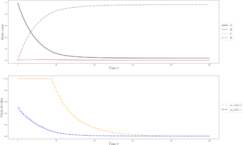  Compartment trajectories and optimal vaccination and social-distancing schedules for a reference solution.

Miscellaneous and Further Reading

The basic reproduction number for the uncontrolled SEIR model is ${{ℛ}}_0=\beta /\gamma$. With the parameters above, ${{ℛ}}_0=5$, corresponding to a highly transmissible pathogen. The two-control formulation combines pharmaceutical intervention (vaccination) with non-pharmaceutical intervention (social distancing), reflecting the dual-measure response used during the COVID-19 pandemic. Necessary optimality conditions via Pontryagin's minimum principle lead to a coupled system of state and adjoint ODEs; the optimal control typically exhibits a bang–singular–bang structure for the vaccination arc and a smooth interior arc for social distancing.

References

[1] Behncke, H. (2000). Optimal control of deterministic epidemics. Optimal Control Applications and Methods, 21(6), 269–285.
[2] Perkins, T. A., & España, G. (2020). Optimal control of the COVID-19 pandemic with non-pharmaceutical interventions. Bulletin of Mathematical Biology, 82, 118.