Tumor Anti Angiogenesis: Difference between revisions
RobertLampel (talk | contribs) |
RobertLampel (talk | contribs) No edit summary |
||
| Line 5: | Line 5: | ||
}} | }} | ||
The '''tumor anti-angiogenesis problem''' is a classical benchmark in biomedical optimal control | The '''tumor anti-angiogenesis problem''' is a classical benchmark in biomedical optimal control. | ||
It is based on the mathematical model of Hahnfeldt et al. [[#Hahnfeldt|[ | It is based on the mathematical model of Hahnfeldt et al. [[#Hahnfeldt|[1]]] for tumor growth under angiogenic signalling, as studied from an optimal control perspective by Ledzewicz and Schättler [[#Ledzewicz|[2]]]. | ||
Angiogenesis is the process by which tumors recruit a network of blood vessels to sustain their growth; anti-angiogenic therapy targets this process by administering inhibitor agents. | Angiogenesis is the process by which tumors recruit a network of blood vessels to sustain their growth; anti-angiogenic therapy targets this process by administering inhibitor agents. | ||
The two biological states are the tumor volume and the carrying capacity of the vascular endothelium (which sets the maximum supportable tumor size). | The two biological states are the tumor volume and the carrying capacity of the vascular endothelium (which sets the maximum supportable tumor size). | ||
A third state tracks the cumulative inhibitor dose, enforcing a total-dose constraint. | A third state tracks the cumulative inhibitor dose, enforcing a total-dose constraint. | ||
The control is the instantaneous inhibitor dose rate. | The control is the instantaneous inhibitor dose rate. | ||
The final time is free and is itself an optimization variable, bounded within a physiologically reasonable range. | |||
The objective is to minimise the tumor volume at the final time. | The objective is to minimise the tumor volume at the final time. | ||
The problem is known to exhibit a rich optimal control structure, including bang–bang arcs, singular arcs, and boundary arcs corresponding to the dose constraint. | The problem is known to exhibit a rich optimal control structure, including bang–bang arcs, singular arcs, and boundary arcs corresponding to the dose constraint. | ||
| Line 19: | Line 20: | ||
<math> | <math> | ||
\begin{array}{lll} | \begin{array}{lll} | ||
\displaystyle \min_{u} && p(t_\mathrm{f}) \\[6pt] | \displaystyle \min_{u,\, t_\mathrm{f}} && p(t_\mathrm{f}) \\[6pt] | ||
\text{subject to} \\ | \text{subject to} \\ | ||
\quad \dot{p}(t) &=& -\xi\, p(t)\,\ln\!\left(\dfrac{p(t)}{q(t)}\right), \\[6pt] | \quad \dot{p}(t) &=& -\xi\, p(t)\,\ln\!\left(\dfrac{p(t)}{q(t)}\right), \\[6pt] | ||
\quad \dot{q}(t) &=& | \quad \dot{q}(t) &=& \bigl(b - \mu - d\, p(t)^{2/3} - G\, u(t)\bigr)\, q(t), \\[6pt] | ||
\quad \dot{y}(t) &=& u(t), \\ | \quad \dot{y}(t) &=& u(t), \\ | ||
\quad (p(0),\, q(0),\, y(0)) &=& (p_0,\, q_0,\, 0), \\ | \quad (p(0),\, q(0),\, y(0)) &=& (p_0,\, q_0,\, 0), \\ | ||
\quad y(t_\mathrm{f}) &\leq& A, \\ | \quad y(t_\mathrm{f}) &\leq& A, \\ | ||
\quad u(t) &\in& [0,\, | \quad u(t) &\in& [0,\, u_{\max}] \quad \forall\, t \in [0, t_\mathrm{f}], \\ | ||
\quad t_\mathrm{f} &\in& [0.5,\, 2.0], | |||
\end{array} | \end{array} | ||
</math> | </math> | ||
| Line 33: | Line 35: | ||
where <math>p(t)</math> is the tumor volume (mm<sup>3</sup>), <math>q(t)</math> is the endothelial carrying capacity (mm<sup>3</sup>), and <math>y(t)</math> is the cumulative inhibitor dose (mg/kg) administered up to time <math>t</math>. | where <math>p(t)</math> is the tumor volume (mm<sup>3</sup>), <math>q(t)</math> is the endothelial carrying capacity (mm<sup>3</sup>), and <math>y(t)</math> is the cumulative inhibitor dose (mg/kg) administered up to time <math>t</math>. | ||
The tumor dynamics follow the Gompertz law <math>\dot{p} = -\xi\,p\ln(p/q)</math>, which models logistic-like growth bounded by the carrying capacity <math>q</math>. | The tumor dynamics follow the Gompertz law <math>\dot{p} = -\xi\,p\ln(p/q)</math>, which models logistic-like growth bounded by the carrying capacity <math>q</math>. | ||
The carrying capacity | The carrying capacity evolves through a balance of self-stimulation (<math>b\,q</math>), natural endothelial cell loss (<math>\mu\,q</math>), inhibition proportional to tumor surface area (<math>d\,p^{2/3}\,q</math>), and drug-induced endothelial loss (<math>G\,u\,q</math>). | ||
The state <math>y(t)</math> enforces the total-dose constraint <math>y(t_\mathrm{f}) \leq A</math> as an isoperimetric inequality. | The state <math>y(t)</math> enforces the total-dose constraint <math>y(t_\mathrm{f}) \leq A</math> as an isoperimetric inequality. | ||
The terminal time <math>t_\mathrm{f}</math> is a free optimization variable. | |||
== Parameters == | == Parameters == | ||
| Line 43: | Line 46: | ||
! Symbol !! Value !! Description | ! Symbol !! Value !! Description | ||
|- | |- | ||
| align=center | <math>\xi</math> || align=right | 0.084 || Tumor growth rate (day<sup>−1</sup>) | | align=center | <math>\xi</math> || align=right | 0.084 || Tumor growth rate (day<sup>−1</sup>) | ||
|- | |- | ||
| align=center | <math>b</math> || align=right | 5.85 || Endothelial | | align=center | <math>b</math> || align=right | 5.85 || Endothelial self-stimulation rate (day<sup>−1</sup>) | ||
|- | |- | ||
| align=center | <math>\mu</math> || align=right | 0 | | align=center | <math>\mu</math> || align=right | 0 || Natural endothelial cell loss rate (day<sup>−1</sup>) | ||
|- | |- | ||
| align=center | <math>d</math> || align=right | 0.00873 || | | align=center | <math>d</math> || align=right | 0.00873 || Angiogenic inhibition coefficient (mm<sup>−2</sup> day<sup>−1</sup>) | ||
|- | |- | ||
| align=center | <math> | | align=center | <math>G</math> || align=right | 0.15 || Drug efficacy on endothelium (kg mg<sup>−1</sup> day<sup>−1</sup>) | ||
|- | |- | ||
| align=center | <math> | | align=center | <math>u_{\max}</math> || align=right | 75 || Maximum inhibitor dose rate (mg kg<sup>−1</sup> day<sup>−1</sup>) | ||
|- | |- | ||
| align=center | <math>A</math> || align=right | | | align=center | <math>A</math> || align=right | 75 || Maximum cumulative inhibitor dose (mg kg<sup>−1</sup>) | ||
|- | |- | ||
| align=center | <math>p_0</math> || align=right | 12000 || Initial tumor volume (mm<sup>3</sup>) | | align=center | <math>p_0</math> || align=right | 12000 || Initial tumor volume (mm<sup>3</sup>) | ||
|- | |- | ||
| align=center | <math>q_0</math> || align=right | 15000 || Initial endothelial carrying capacity (mm<sup>3</sup>) | | align=center | <math>q_0</math> || align=right | 15000 || Initial endothelial carrying capacity (mm<sup>3</sup>) | ||
|- | |- | ||
| align=center | <math>t_\mathrm{f}</math> || align=right | | | align=center | <math>t_\mathrm{f}</math> || align=right | free || Terminal time, optimized in [0.5, 2.0] (days) | ||
|} | |} | ||
| Line 69: | Line 72: | ||
<gallery caption="Reference solution plots" widths="500px" heights="300px" perrow="1"> | <gallery caption="Reference solution plots" widths="500px" heights="300px" perrow="1"> | ||
Image: Tumor_Anti_Angiogenesis.png | Tumor volume, carrying capacity, cumulative dose, and optimal inhibitor schedule for a reference solution. | Image:Tumor_Anti_Angiogenesis.png| Tumor volume, carrying capacity, cumulative dose, and optimal inhibitor schedule for a reference solution. | ||
</gallery> | </gallery> | ||
| Line 75: | Line 78: | ||
The equilibrium <math>p^* = q^*</math> corresponds to a tumor at maximum sustainable size. | The equilibrium <math>p^* = q^*</math> corresponds to a tumor at maximum sustainable size. | ||
Without treatment, <math>p(t)</math> converges to this steady state. | Without treatment, <math>p(t)</math> converges to this steady state. | ||
Ledzewicz and Schättler [[#Ledzewicz|[ | Ledzewicz and Schättler [[#Ledzewicz|[2]]] characterise the optimal control using Pontryagin's minimum principle and show that the optimal policy consists of a sequence of full-dose (<math>u = u_{\max}</math>), no-dose (<math>u = 0</math>), and singular arcs, depending on the initial conditions and remaining dose budget. | ||
The problem is included in the GPOPS-II benchmark suite [[#Patterson|[3]]]. | |||
== References == | == References == | ||
<span id=" | <span id="Hahnfeldt">[1]</span> Hahnfeldt, P., Panigrahy, D., Folkman, J., & Hlatky, L. (1999). Tumor development under angiogenic signaling: A dynamical theory of tumor growth, treatment response, and postvascular dormancy. <i>Cancer Research</i>, 59(19), 4770–4775.<br> | ||
<span id="Ledzewicz">[2]</span> Ledzewicz, U., & Schättler, H. (2007). Antiangiogenic therapy in cancer treatment as an optimal control problem. <i>SIAM Journal on Control and Optimization</i>, 46(3), 1052–1079.<br> | |||
<span id="Ledzewicz">[ | <span id="Patterson">[3]</span> Patterson, M. A., & Rao, A. V. (2014). GPOPS-II: A MATLAB software for solving multiple-phase optimal control problems using hp-adaptive Gaussian quadrature collocation methods and sparse nonlinear programming. <i>ACM Transactions on Mathematical Software</i>, 41(1), 1.<br> | ||
[[Category:MIOCP]] | [[Category:MIOCP]] | ||
[[Category:ODE model]] | [[Category:ODE model]] | ||
[[Category:Singular arc]] | [[Category:Singular arc]] | ||
[[Category:Free terminal time]] | |||
Latest revision as of 11:30, 4 September 2026
| Tumor Anti Angiogenesis | |
|---|---|
| State dimension: | 1 |
| Differential states: | 3 |
| Discrete control functions: | 1 |
The tumor anti-angiogenesis problem is a classical benchmark in biomedical optimal control.
It is based on the mathematical model of Hahnfeldt et al. [1] for tumor growth under angiogenic signalling, as studied from an optimal control perspective by Ledzewicz and Schättler [2]. Angiogenesis is the process by which tumors recruit a network of blood vessels to sustain their growth; anti-angiogenic therapy targets this process by administering inhibitor agents. The two biological states are the tumor volume and the carrying capacity of the vascular endothelium (which sets the maximum supportable tumor size). A third state tracks the cumulative inhibitor dose, enforcing a total-dose constraint. The control is the instantaneous inhibitor dose rate. The final time is free and is itself an optimization variable, bounded within a physiologically reasonable range. The objective is to minimise the tumor volume at the final time. The problem is known to exhibit a rich optimal control structure, including bang–bang arcs, singular arcs, and boundary arcs corresponding to the dose constraint.
Mathematical formulation
where is the tumor volume (mm3), is the endothelial carrying capacity (mm3), and is the cumulative inhibitor dose (mg/kg) administered up to time . The tumor dynamics follow the Gompertz law , which models logistic-like growth bounded by the carrying capacity . The carrying capacity evolves through a balance of self-stimulation (), natural endothelial cell loss (), inhibition proportional to tumor surface area (), and drug-induced endothelial loss (). The state enforces the total-dose constraint as an isoperimetric inequality. The terminal time is a free optimization variable.
Parameters
These fixed values are used within the model:
| Symbol | Value | Description |
|---|---|---|
| 0.084 | Tumor growth rate (day−1) | |
| 5.85 | Endothelial self-stimulation rate (day−1) | |
| 0 | Natural endothelial cell loss rate (day−1) | |
| 0.00873 | Angiogenic inhibition coefficient (mm−2 day−1) | |
| 0.15 | Drug efficacy on endothelium (kg mg−1 day−1) | |
| 75 | Maximum inhibitor dose rate (mg kg−1 day−1) | |
| 75 | Maximum cumulative inhibitor dose (mg kg−1) | |
| 12000 | Initial tumor volume (mm3) | |
| 15000 | Initial endothelial carrying capacity (mm3) | |
| free | Terminal time, optimized in [0.5, 2.0] (days) |
Reference Solutions
Here is one local solution to the above control problem.
- Reference solution plots
-
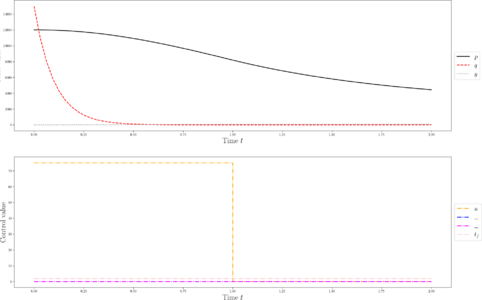 Tumor volume, carrying capacity, cumulative dose, and optimal inhibitor schedule for a reference solution.

Miscellaneous and Further Reading
The equilibrium corresponds to a tumor at maximum sustainable size. Without treatment, converges to this steady state. Ledzewicz and Schättler [2] characterise the optimal control using Pontryagin's minimum principle and show that the optimal policy consists of a sequence of full-dose (), no-dose (), and singular arcs, depending on the initial conditions and remaining dose budget. The problem is included in the GPOPS-II benchmark suite [3].
References
[1] Hahnfeldt, P., Panigrahy, D., Folkman, J., & Hlatky, L. (1999). Tumor development under angiogenic signaling: A dynamical theory of tumor growth, treatment response, and postvascular dormancy. Cancer Research, 59(19), 4770–4775.
[2] Ledzewicz, U., & Schättler, H. (2007). Antiangiogenic therapy in cancer treatment as an optimal control problem. SIAM Journal on Control and Optimization, 46(3), 1052–1079.
[3] Patterson, M. A., & Rao, A. V. (2014). GPOPS-II: A MATLAB software for solving multiple-phase optimal control problems using hp-adaptive Gaussian quadrature collocation methods and sparse nonlinear programming. ACM Transactions on Mathematical Software, 41(1), 1.