Difference between revisions of "Car testdrive (lane change manoeuvre)"
(→Test course) |
FelixMueller (Talk | contribs) |
||
| (13 intermediate revisions by 4 users not shown) | |||
| Line 4: | Line 4: | ||
|nu = 3 | |nu = 3 | ||
|nw = 1 | |nw = 1 | ||
| + | |nc = 1 | ||
|nri = 7 | |nri = 7 | ||
}} | }} | ||
| − | The | + | The testdrive control problem is a time optimal double lane change maneouvre with gear shift. It has been introduced as a benchmark problem for mixed-integer optimal control by <bib id="Gerdts2005" />. |
| − | + | ||
| − | + | ||
== Mathematical formulation == | == Mathematical formulation == | ||
| − | + | The mathematical equations form a small-scale [[:Category:ODE model|ODE model]]. | |
| + | |||
| + | The vehicle dynamics are based on a single-track model, derived under the simplifying assumption that rolling and pitching of the car body can be neglected. Consequentially, only a single front and rear wheel is modeled, located in the virtual center of the original two wheels. Motion of the car body is considered on the horizontal plane only. | ||
Four controls represent the driver's choice on steering and velocity. We denote with <math>w_\delta</math> the steering wheel's angular velocity. The force <math>F_\text{B}</math> controls the total braking force, while the accelerator pedal position <math>\phi</math> is translated into an accelerating force. Finally, the selected gear <math>\mu</math> influences the effective engine torque's transmission. | Four controls represent the driver's choice on steering and velocity. We denote with <math>w_\delta</math> the steering wheel's angular velocity. The force <math>F_\text{B}</math> controls the total braking force, while the accelerator pedal position <math>\phi</math> is translated into an accelerating force. Finally, the selected gear <math>\mu</math> influences the effective engine torque's transmission. | ||
| + | |||
| + | |||
== Resulting MIOCP == | == Resulting MIOCP == | ||
| Line 24: | Line 27: | ||
\begin{array}{llcl} | \begin{array}{llcl} | ||
\displaystyle \min_{x(\cdot), u(\cdot), \mu(\cdot)} & t_\text{f} \\[1.5ex] | \displaystyle \min_{x(\cdot), u(\cdot), \mu(\cdot)} & t_\text{f} \\[1.5ex] | ||
| − | \mbox{s.t.} & \dot{x} | + | \mbox{s.t.} & \dot{x} & = & f(t, x, u, \mu), \\ |
& x(t_0) &=& x_0, \\ | & x(t_0) &=& x_0, \\ | ||
| − | & r(t,x | + | & r(t,x,u) &\geq& 0, \\ |
& \mu(t) &\in& \{1, 2, 3, 4, 5\}. | & \mu(t) &\in& \{1, 2, 3, 4, 5\}. | ||
\end{array} | \end{array} | ||
| Line 35: | Line 38: | ||
These fixed values are used within the model. | These fixed values are used within the model. | ||
| − | + | {| border="1" align="center" cellpadding="5" cellspacing="0" | |
| − | + | |- bgcolor=#c7c7c7 | |
| − | + | ! Symbol !! Value !! Unit !! Description | |
| − | + | |- | |
| − | + | | align=center | <math>m</math> || align=right | 1.239e+3 || kg || Mass of the car | |
| − | + | |- | |
| − | + | | align=center | <math>g</math> || align=right | 9.81 || m/s^2 || Gravity constant | |
| − | + | |- | |
| − | + | | align=center | <math>l_\text{f}</math> || align=right | 1.19016 || m || Front wheel distance to center of gravity | |
| − | + | |- | |
| − | + | | align=center | <math>l_\text{r}</math> || align=right | 1.37484 || m || Rear wheel distance to center of gravity | |
| − | + | |- | |
| − | + | | align=center | <math>e_\text{SP}</math> || align=right | 0.5 || m || Drag mount point distance to center of gravity | |
| − | + | |- | |
| − | + | | align=center | <math>R</math> || align=right | 0.302 || m || Wheel radius | |
| − | + | |- | |
| − | + | | align=center | <math>I_\text{zz}</math> || align=right | 1.752e+3 || kg m^2 || Moment of inertia | |
| − | + | |- | |
| − | + | | align=center | <math>c_\text{w}</math> || align=right | 0.3 || - || Air drag coefficient | |
| − | + | |- | |
| − | + | | align=center | <math>\varrho</math> || align=right | 1.249512 || kg/m^3 || Air density | |
| − | + | |- | |
| − | + | | align=center | <math>A</math> || align=right | 1.4378946874 || m^2 || Effective flow surface | |
| − | + | |- | |
| − | + | | align=center | <math>i_\text{g}</math> || align=right | 3.09, 2.002, 1.33, 1.0, 0.805 || - || Transmission ratios for the five gears | |
| − | + | |- | |
| − | + | | align=center | <math>i_\text{t}</math> || align=right | 3.91 || - || Engine transmission ratio | |
| − | + | |- | |
| − | + | | align=center | <math>B_\text{f}</math> || align=right | 1.096e+1 || - || Pacejka coefficients (stiffness) | |
| − | + | |- | |
| + | | align=center | <math>B_\text{r}</math> || align=right | 1.267e+1 || - || | ||
| + | |- | ||
| + | | align=center | <math>C_\text{f}</math> || align=right | 1.3 || - || Pacejka coefficients (shape) | ||
| + | |- | ||
| + | | align=center | <math>C_\text{r}</math> || align=right | 1.3 || - || | ||
| + | |- | ||
| + | | align=center | <math>D_\text{f}</math> || align=right | 4.5604e+3 || - || Pacejka coefficients (peak) | ||
| + | |- | ||
| + | | align=center | <math>D_\text{r}</math> || align=right | 3.94781e+3 || - || | ||
| + | |- | ||
| + | | align=center | <math>E_\text{f}</math> || align=right | -0.5 || - || Pacejka coefficients (curvature) | ||
| + | |- | ||
| + | | align=center | <math>E_\text{r}</math> || align=right | -0.5 || - || | ||
| + | |} | ||
== Test course == | == Test course == | ||
| − | The double-lane change manoeuvre presented in < | + | The double-lane change manoeuvre presented in <bib id="Gerdts2005" /> is realized by constraining the car's position onto a prescribed track at any time <math>t\in[t_0,t_\text{f}]</math>. Starting in the left position with an initial prescribed velocity, the driver is asked to manage a change of lanes modeled by an offset of 3.5 meters in the track. Afterwards he is asked to return to the starting lane. This manoeuvre can be regarded as an overtaking move or as an evasive action taken to avoid hitting an obstacle suddenly appearing on the starting lane. |
From a mathematical point of view, the test track is described by setting up piecewise cubic spline functions <math>P_\text{l}(x)</math> and <math>P_\text{r}(x)</math> modeling the top and bottom track boundary, given a horizontal position <math>x</math>. | From a mathematical point of view, the test track is described by setting up piecewise cubic spline functions <math>P_\text{l}(x)</math> and <math>P_\text{r}(x)</math> modeling the top and bottom track boundary, given a horizontal position <math>x</math>. | ||
| Line 106: | Line 123: | ||
</math> | </math> | ||
| − | [[Image:test-course.png]] | + | [[Image:test-course.png|Test course for the double lane change manoeuvre]] |
== Reference Solutions == | == Reference Solutions == | ||
| − | Reference solutions for the case of a fixed time-grid are given in < | + | Reference solutions for the case of a fixed time-grid are given in <bib id="Gerdts2005" />. Solutions for a non-fixed time grid are given in <bib id="Gerdts2006" />. |
== Source Code == | == Source Code == | ||
| − | + | Model descriptions are available in | |
| + | |||
| + | * [[:Category:Muscod | Muscod code]] at [[Car testdrive (lane change manoeuvre) (Muscod)]] | ||
== Variants == | == Variants == | ||
| Line 121: | Line 140: | ||
== References == | == References == | ||
| − | < | + | <biblist /> |
<!--List of all categories this page is part of. List characterization of solution behavior, model properties, ore presence of implementation details (e.g., AMPL for AMPL model) here --> | <!--List of all categories this page is part of. List characterization of solution behavior, model properties, ore presence of implementation details (e.g., AMPL for AMPL model) here --> | ||
Latest revision as of 10:25, 27 July 2016
| Car testdrive (lane change manoeuvre) | |
|---|---|
| State dimension: | 1 |
| Differential states: | 7 |
| Continuous control functions: | 3 |
| Discrete control functions: | 1 |
| Path constraints: | 1 |
| Interior point inequalities: | 7 |
The testdrive control problem is a time optimal double lane change maneouvre with gear shift. It has been introduced as a benchmark problem for mixed-integer optimal control by [Gerdts2005]Author: M. Gerdts
Journal: Optimal Control Applications and Methods
Pages: 1--18
Title: Solving mixed-integer optimal control problems by Branch\&Bound: A case study from automobile test-driving with gear shift
Volume: 26
Year: 2005 .
.
Contents
Mathematical formulation
The mathematical equations form a small-scale ODE model.
The vehicle dynamics are based on a single-track model, derived under the simplifying assumption that rolling and pitching of the car body can be neglected. Consequentially, only a single front and rear wheel is modeled, located in the virtual center of the original two wheels. Motion of the car body is considered on the horizontal plane only.
Four controls represent the driver's choice on steering and velocity. We denote with  the steering wheel's angular velocity. The force
  controls the total braking force, while the accelerator pedal position
  is translated into an accelerating force. Finally, the selected gear
  influences the effective engine torque's transmission.
Resulting MIOCP
For ![t \in [t_0, t_f]](https://mintoc.de/images/math/5/5/8/55823791d9100bcb5461801aff4f6edd.png) almost everywhere the mixed-integer optimal control problem is given by
almost everywhere the mixed-integer optimal control problem is given by
![\begin{array}{llcl}
\displaystyle \min_{x(\cdot), u(\cdot), \mu(\cdot)} & t_\text{f} \\[1.5ex]
\mbox{s.t.} & \dot{x} & = & f(t, x, u, \mu), \\
& x(t_0) &=& x_0, \\
& r(t,x,u) &\geq& 0, \\
& \mu(t) &\in& \{1, 2, 3, 4, 5\}.
\end{array}](https://mintoc.de/images/math/3/7/2/37233d15e732884f1b7a1799a1069e03.png)
Parameters
These fixed values are used within the model.
| Symbol | Value | Unit | Description |
|---|---|---|---|
 |
1.239e+3 | kg | Mass of the car |
 |
9.81 | m/s^2 | Gravity constant |
 |
1.19016 | m | Front wheel distance to center of gravity |
 |
1.37484 | m | Rear wheel distance to center of gravity |
 |
0.5 | m | Drag mount point distance to center of gravity |
 |
0.302 | m | Wheel radius |
 |
1.752e+3 | kg m^2 | Moment of inertia |
 |
0.3 | - | Air drag coefficient |
 |
1.249512 | kg/m^3 | Air density |
 |
1.4378946874 | m^2 | Effective flow surface |
 |
3.09, 2.002, 1.33, 1.0, 0.805 | - | Transmission ratios for the five gears |
 |
3.91 | - | Engine transmission ratio |
 |
1.096e+1 | - | Pacejka coefficients (stiffness) |
 |
1.267e+1 | - | |
 |
1.3 | - | Pacejka coefficients (shape) |
 |
1.3 | - | |
 |
4.5604e+3 | - | Pacejka coefficients (peak) |
 |
3.94781e+3 | - | |
 |
-0.5 | - | Pacejka coefficients (curvature) |
 |
-0.5 | - |
Test course
The double-lane change manoeuvre presented in [Gerdts2005]Author: M. Gerdts
Journal: Optimal Control Applications and Methods
Pages: 1--18
Title: Solving mixed-integer optimal control problems by Branch\&Bound: A case study from automobile test-driving with gear shift
Volume: 26
Year: 2005 is realized by constraining the car's position onto a prescribed track at any time ![t\in[t_0,t_\text{f}]](https://mintoc.de/images/math/e/2/3/e234c61ce225d19679331caf0281c8b0.png) . Starting in the left position with an initial prescribed velocity, the driver is asked to manage a change of lanes modeled by an offset of 3.5 meters in the track. Afterwards he is asked to return to the starting lane. This manoeuvre can be regarded as an overtaking move or as an evasive action taken to avoid hitting an obstacle suddenly appearing on the starting lane.
. Starting in the left position with an initial prescribed velocity, the driver is asked to manage a change of lanes modeled by an offset of 3.5 meters in the track. Afterwards he is asked to return to the starting lane. This manoeuvre can be regarded as an overtaking move or as an evasive action taken to avoid hitting an obstacle suddenly appearing on the starting lane.
From a mathematical point of view, the test track is described by setting up piecewise cubic spline functions  and
and  modeling the top and bottom track boundary, given a horizontal position
  .
.
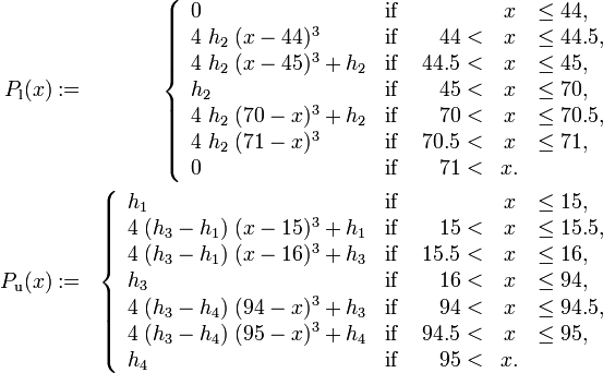
where  is the car's width and


Reference Solutions
Reference solutions for the case of a fixed time-grid are given in [Gerdts2005]Author: M. Gerdts
Journal: Optimal Control Applications and Methods
Pages: 1--18
Title: Solving mixed-integer optimal control problems by Branch\&Bound: A case study from automobile test-driving with gear shift
Volume: 26
Year: 2005. Solutions for a non-fixed time grid are given in [Gerdts2006]Author: M. Gerdts
Journal: Optimal Control Applications and Methods
Number: 3
Pages: 169--182
Title: A variable time transformation method for mixed-integer optimal control problems
Volume: 27
Year: 2006.
Source Code
Model descriptions are available in
Variants
See testdrive overview page.
References
There were no citations found in the article.