Difference between revisions of "Lotka Experimental Design"
(first crappy version, need to save to restart server) |
(Model description is complete) |
||
| Line 23: | Line 23: | ||
</math> | </math> | ||
</p> | </p> | ||
| − | where <math>u(\cdot)</math> is a fishing control that may or may not be fixed. The other parameters, the initial values and <math>t_f = 12</math> are fixed. We are interested in how to fish and when to measure, with an upper bound <math>M</math> on the measuring time. We can measure the states directly, <math>h^1(x(t)) = x_1(t)</math> and <math>h^2(x(t)) = x_2(t)</math>. We use two different sampling functions, <math>w^1(\cdot)</math> and <math>w^2(\cdot)</math> in the same experimental setting. This can be seen either as a two-dimensional measurement function <math>h(x(t))</math>, or as a special case of a multiple experiment, in which <math>u(\cdot), x(\cdot)</math>, and <math> | + | where <math>u(\cdot)</math> is a fishing control that may or may not be fixed. The other parameters, the initial values and <math>t_f = 12</math> are fixed. We are interested in how to fish and when to measure, with an upper bound <math>M</math> on the measuring time. We can measure the states directly, <math>h^1(x(t)) = x_1(t)</math> and <math>h^2(x(t)) = x_2(t)</math>. We use two different sampling functions, <math>w^1(\cdot)</math> and <math>w^2(\cdot)</math> in the same experimental setting. This can be seen either as a two-dimensional measurement function <math>h(x(t))</math>, or as a special case of a multiple experiment, in which <math>u(\cdot), x(\cdot)</math>, and <math>G(\cdot)</math> are identical. The experimental design problem then reads |
| − | + | ||
| − | + | ||
| − | + | ||
<p> | <p> | ||
<math> | <math> | ||
| − | \begin{array}{ | + | \begin{array}{lll} |
| − | \displaystyle \min_{x, w} & | + | \displaystyle \min_{x,G,F,z^1,z^2,u,w^1,w^2} && \text{trace} \; \left( F^{-1}(t_f) \right) \\ |
| − | \ | + | \text{subject to} \\ |
| − | + | \quad \dot{x_1}(t) & = & p_1 \; x_1(t) - p_2 x_1(t) x_2(t) - p_5 u(t) x_1(t),\\ | |
| − | + | \quad \dot{x_2}(t) & = & - p_3 \; x_2(t) + p_4 x_1(t) x_2(t) - p_6 u(t) x_2(t),\\ | |
| − | + | \quad \dot{G_{11}}(t) & = & f_{x11}(\cdot) \; G_{11}(t) + f_{x12}(\cdot) \; G_{21}(t) + f_{p12}(\cdot), \\ | |
| − | + | \quad \dot{G_{12}}(t) & = & f_{x11}(\cdot) \; G_{12}(t) + f_{x12}(\cdot) \; G_{22}(t), \\ | |
| − | \end{array} | + | \quad \dot{G_{21}}(t) & = & f_{x21}(\cdot) \; G_{11}(t) + f_{x22}(\cdot) \; G_{21}(t), \\ |
| + | \quad \dot{G_{22}}(t) & = & f_{x21}(\cdot) \; G_{12}(t) + f_{x22}(\cdot) \; G_{22}(t) + f_{p24}(\cdot), \\ | ||
| + | \quad \dot{F_{11}}(t) & = & w^1(t) G_{11}(t)^2 + w^2(t) G_{12}(t)^2, \\ | ||
| + | \quad \dot{F_{12}}(t) & = & w^1(t) G_{11}(t) G_{12}(t) + w^2(t) G_{12}(t) G_{22}(t), \\ | ||
| + | \quad \dot{F_{22}}(t) & = & w^1(t) G_{21}(t)^2 + w^2(t) G_{22}(t)^2, \\ | ||
| + | \quad \dot{z^1}(t) & = & w^1(t), \\ | ||
| + | \quad \dot{z^2}(t) & = & w^2(t), \\[1.5ex] | ||
| + | \quad x(0) &=& (0.5, 0.7), \\ | ||
| + | \quad G(0) &=& F(0) = 0, \\ | ||
| + | \quad z^1(0) &=& z^2(0) = 0, \\ [1.5ex] | ||
| + | \quad u(t) & \in & \mathcal{U}, \; w^1(t) \in \mathcal{W}, \; w^2(t) \in \mathcal{W}, \\ | ||
| + | \quad 0 & \le & M - z(t_f) | ||
| + | \end{array} | ||
</math> | </math> | ||
</p> | </p> | ||
| − | + | with | |
| + | <math>f_{x11}(\cdot) = \partial f_1(\cdot) / \partial x_1 = p_1 - p_2 x_2(t) - p_5 u(t)</math>, | ||
| + | <math>f_{x12}(\cdot) = - p_2 x_1(t)</math>, | ||
| + | <math>f_{x21}(\cdot) = p_4 x_2(t)</math>, | ||
| + | <math>f_{x22}(\cdot) = -p_3 + p_4 x_1(t) - p_6 u(t)</math>, and | ||
| + | <math>f_{p12}(\cdot) = \partial f_1(\cdot) / \partial p_2 = -x_1(t) x_2(t)</math>, | ||
| + | <math>f_{p24}(\cdot) = \partial f_2(\cdot) / \partial p_4 = x_1(t) x_2(t)</math>. | ||
| + | |||
| + | Note that the state <math>F_{21}(\cdot) = F_{12}(\cdot)</math> has been left out for reasons of symmetry. | ||
== Parameters == | == Parameters == | ||
| − | + | We use <math>t_f=12</math>, <math>p_1 = p_2 = p_3 = p_4 = 1</math>, and <math>p_5 = 0.4</math>, <math>p_6 = 0.2</math>. The upper bound on the measurement time intervals is chosen as <math>M=4</math>. | |
| − | + | ||
| − | <math> | + | |
| − | + | ||
| − | + | ||
| − | + | ||
| − | + | ||
| − | </math> | + | |
== Reference Solutions == | == Reference Solutions == | ||
| − | + | bla | |
| − | + | ||
| − | + | ||
<gallery caption="Reference solution plots" widths="180px" heights="140px" perrow="2"> | <gallery caption="Reference solution plots" widths="180px" heights="140px" perrow="2"> | ||
| Line 79: | Line 87: | ||
* a prescribed time grid for the control function <bibref>Sager2006</bibref>, see also [[Lotka Experimental Design (AMPL)]], | * a prescribed time grid for the control function <bibref>Sager2006</bibref>, see also [[Lotka Experimental Design (AMPL)]], | ||
| + | * no fishing, i.e., <math>u \equiv 0</math>, | ||
* different fishing control functions for the two species, | * different fishing control functions for the two species, | ||
* different parameters and start values. | * different parameters and start values. | ||
Revision as of 10:13, 31 August 2012
| Lotka Experimental Design | |
|---|---|
| State dimension: | 1 |
| Differential states: | 12 |
| Discrete control functions: | 2 |
| Interior point equalities: | 12 |
The Lotka Experimental Design problem looks for an optimal fishing strategy to be performed on a fixed time horizon to control the biomasses of both predator as prey fish as described in Lotka Volterra fishing problem. The goal here, however, is to minimize the uncertainty of a follow-up parameter estimation problem. In addition to the fishing decision the question when measurements of the two state variables are performed becomes a degree of freedom.
The mathematical equations form a small-scale ODE model. The ODE from Lotka Volterra fishing problem is extended such that it also includes state sensitivities, the Fisher information matrix entries and integrated sampling states.
The optimal integer control functions shows bang bang behavior.
Contents
Mathematical formulation
We are interested in estimating the parameters  and
and  of the Lotka-Volterra type predator-prey fish initial value problem
![\begin{array}{rcl}
\dot{x_1}(t) &=& p_1 \; x_1(t) - p_2 x_1(t) x_2(t) - p_5 u(t) x_1(t), \; t \in [0,t_f], \quad x_1(0) = 0.5, \\
\dot{x_2}(t) &=& - p_3 \; x_2(t) + p_4 x_1(t) x_2(t) - p_6 u(t) x_2(t), \; t \in [0,t_f], \quad x_2(0) = 0.7,
\end{array}](https://mintoc.de/images/math/3/1/d/31daaad30b442898b092905f1c6b6f93.png)
where  is a fishing control that may or may not be fixed. The other parameters, the initial values and
  are fixed. We are interested in how to fish and when to measure, with an upper bound
  on the measuring time. We can measure the states directly,
  and
and  . We use two different sampling functions,
  and
and  in the same experimental setting. This can be seen either as a two-dimensional measurement function
  , or as a special case of a multiple experiment, in which
  , and
, and  are identical. The experimental design problem then reads
![\begin{array}{lll}
\displaystyle \min_{x,G,F,z^1,z^2,u,w^1,w^2} && \text{trace} \; \left( F^{-1}(t_f) \right) \\
\text{subject to} \\
\quad \dot{x_1}(t) & = & p_1 \; x_1(t) - p_2 x_1(t) x_2(t) - p_5 u(t) x_1(t),\\
\quad \dot{x_2}(t) & = & - p_3 \; x_2(t) + p_4 x_1(t) x_2(t) - p_6 u(t) x_2(t),\\
\quad \dot{G_{11}}(t) & = & f_{x11}(\cdot) \; G_{11}(t) + f_{x12}(\cdot) \; G_{21}(t) + f_{p12}(\cdot), \\
\quad \dot{G_{12}}(t) & = & f_{x11}(\cdot) \; G_{12}(t) + f_{x12}(\cdot) \; G_{22}(t), \\
\quad \dot{G_{21}}(t) & = & f_{x21}(\cdot) \; G_{11}(t) + f_{x22}(\cdot) \; G_{21}(t), \\
\quad \dot{G_{22}}(t) & = & f_{x21}(\cdot) \; G_{12}(t) + f_{x22}(\cdot) \; G_{22}(t) + f_{p24}(\cdot), \\
\quad \dot{F_{11}}(t) & = & w^1(t) G_{11}(t)^2 + w^2(t) G_{12}(t)^2, \\
\quad \dot{F_{12}}(t) & = & w^1(t) G_{11}(t) G_{12}(t) + w^2(t) G_{12}(t) G_{22}(t), \\
\quad \dot{F_{22}}(t) & = & w^1(t) G_{21}(t)^2 + w^2(t) G_{22}(t)^2, \\
\quad \dot{z^1}(t) & = & w^1(t), \\
\quad \dot{z^2}(t) & = & w^2(t), \\[1.5ex]
\quad x(0) &=& (0.5, 0.7), \\
\quad G(0) &=& F(0) = 0, \\
\quad z^1(0) &=& z^2(0) = 0, \\ [1.5ex]
\quad u(t) & \in & \mathcal{U}, \; w^1(t) \in \mathcal{W}, \; w^2(t) \in \mathcal{W}, \\
\quad 0 & \le & M - z(t_f)
\end{array}](https://mintoc.de/images/math/4/c/4/4c4ffea7ba3916530564b6cc2c84c371.png)
with
 ,
,
 ,
,
 ,
,
 , and
, and
 ,
,
 .
.
Note that the state  has been left out for reasons of symmetry.
Parameters
We use , 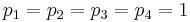 , and
, and  ,
,  . The upper bound on the measurement time intervals is chosen as
  .
.
Reference Solutions
bla
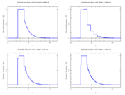
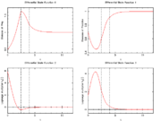
- Reference solution plots
Optimal relaxed control determined by an indirect approach and by a direct approach on different control discretization grids.
Differential states and corresponding adjoint variables in the indirect approach.
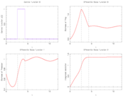
Control and differential states with only two switches.
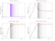
Control and differential states with 56 switches.


Source Code
Model descriptions are available in
Variants
There are several alternative formulations and variants of the above problem, in particular
- a prescribed time grid for the control function <bibref>Sager2006</bibref>, see also Lotka Experimental Design (AMPL),
- no fishing, i.e.,
 ,
, - different fishing control functions for the two species,
- different parameters and start values.
Miscellaneous and Further Reading
The Lotka Volterra fishing problem was introduced by Sebastian Sager in a proceedings paper <bibref>Sager2006</bibref> and revisited in his PhD thesis <bibref>Sager2005</bibref>. These are also the references to look for more details. The experimental design problem has been described in the habilitation thesis of Sager, <bibref>Sager2011d</bibref>.
References
<bibreferences/>