Difference between revisions of "Lotka Volterra Multimode fishing problem"
ClemensZeile (Talk | contribs) |
ClemensZeile (Talk | contribs) |
||
| Line 44: | Line 44: | ||
== Reference Solutions == | == Reference Solutions == | ||
| − | If the problem is relaxed, i.e., we demand that <math>w(t)</math> be in the continuous interval <math>[0, 1]</math> instead of the binary choice <math>\{0,1\}</math>, the optimal solution can be determined by means of | + | If the problem is relaxed, i.e., we demand that <math>w(t)</math> be in the continuous interval <math>[0, 1]</math> instead of the binary choice <math>\{0,1\}</math>, the optimal solution can be determined by means of direct optimal control. |
| − | The optimal objective value of | + | The optimal objective value of the relaxed problem with <math> n_t=12000, \, n_u=400 </math> is <math>x_2(t_f) =1.82875272</math>. The objective value of the binary controls obtained by Combinatorial Integral Approimation (CIA) is <math>x_2(t_f) =1.82878681</math>. |
<gallery caption="Reference solution plots" widths="180px" heights="140px" perrow="2"> | <gallery caption="Reference solution plots" widths="180px" heights="140px" perrow="2"> | ||
| − | Image: | + | Image:MmlotkaRelaxed_12000_30_1.png| Optimal relaxed controls and states determined by an direct approach with ampl_mintoc (Radau collocation) and <math>n_t=12000, \, n_u=400</math>. |
| − | + | Image:MmlotkaCIA 12000 30 1.png| Optimal binary controls and states determined by an direct approach (Radau collocation) with ampl_mintoc and <math>n_t=12000, \, n_u=400</math>. The relaxed controls were approximated by Combinatorial Integral Approximation. | |
| − | Image: | + | |
| − | + | ||
</gallery> | </gallery> | ||
Latest revision as of 14:16, 21 December 2017
| Lotka Volterra Multimode fishing problem | |
|---|---|
| State dimension: | 1 |
| Differential states: | 3 |
| Discrete control functions: | 3 |
| Interior point equalities: | 3 |
This site describes a Lotka Volterra variant with three binary controls instead of only one control.
Mathematical formulation
The mixed-integer optimal control problem is given by
![\begin{array}{llclr}
\displaystyle \min_{x, w} & x_2(t_f) \\[1.5ex]
\mbox{s.t.}
& \dot{x}_0 & = & x_0 - x_0 x_1 - \; \sum\limits_{i=1}^{3} c_{0,i}\; x_0 \; w_i, \\
& \dot{x}_1 & = & - x_1 + x_0 x_1 - \; \sum\limits_{i=1}^{3} c_{1,i}\; x_1 \; w_i, \\
& \dot{x}_2 & = & (x_0 - 1)^2 + (x_1 - 1)^2, \\[1.5ex]
& x(0) &=& (0.5, 0.7, 0)^T, \\
& \sum\limits_{i=1}^{3}w_i(t) &=& 1, \\
& w_i(t) &\in& \{0, 1\}, \quad i=1\ldots 3.
\end{array}](https://mintoc.de/images/math/d/a/d/dad7be9264b08357bd97039bd5e954d2.png)
Here the differential states  describe the biomasses of prey and predator, respectively. The third differential state is used here to transform the objective, an integrated deviation, into the Mayer formulation
  . This problem variant allows to choose between three different fishing options.
Parameters
These fixed values are used within the model.
![\begin{array}{rcl}
[t_0, t_f] &=& [0, 12],\\
(c_{0,1}, c_{1,1}) &=& (0.2, 0.1),\\
(c_{0,2}, c_{1,2}) &=& (0.4, 0.2),\\
(c_{0,3}, c_{1,3}) &=& (0.01, 0.1).
\end{array}](https://mintoc.de/images/math/7/3/d/73dd5018bea7b43a28e8854d28fc9436.png)
Reference Solutions
If the problem is relaxed, i.e., we demand that  be in the continuous interval
 ![[0, 1]](https://mintoc.de/images/math/c/c/f/ccfcd347d0bf65dc77afe01a3306a96b.png) instead of the binary choice
instead of the binary choice  , the optimal solution can be determined by means of direct optimal control.
The optimal objective value of the relaxed problem with  is
is  . The objective value of the binary controls obtained by Combinatorial Integral Approimation (CIA) is
  .
.
- Reference solution plots
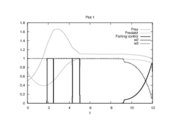
Optimal relaxed controls and states determined by an direct approach with ampl_mintoc (Radau collocation) and
.
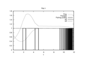
Optimal binary controls and states determined by an direct approach (Radau collocation) with ampl_mintoc and
. The relaxed controls were approximated by Combinatorial Integral Approximation.

