Lotka Volterra Multimode fishing problem
| Lotka Volterra Multimode fishing problem | |
|---|---|
| State dimension: | 1 |
| Differential states: | 3 |
| Discrete control functions: | 3 |
| Interior point equalities: | 3 |
This site describes a Lotka Volterra variant with three binary controls instead of only one control.
Mathematical formulation
The mixed-integer optimal control problem is given by
![\begin{array}{llclr}
\displaystyle \min_{x, w} & x_2(t_f) \\[1.5ex]
\mbox{s.t.}
& \dot{x}_0 & = & x_0 - x_0 x_1 - \; \sum\limits_{i=1}^{3} c_{0,i}\; x_0 \; w_i, \\
& \dot{x}_1 & = & - x_1 + x_0 x_1 - \; \sum\limits_{i=1}^{3} c_{1,i}\; x_1 \; w_i, \\
& \dot{x}_2 & = & (x_0 - 1)^2 + (x_1 - 1)^2, \\[1.5ex]
& x(0) &=& (0.5, 0.7, 0)^T, \\
& \sum\limits_{i=1}^{3}w_i(t) &=& 1, \\
& w_i(t) &\in& \{0, 1\}, \quad i=1\ldots 3.
\end{array}](https://mintoc.de/images/math/d/a/d/dad7be9264b08357bd97039bd5e954d2.png)
Here the differential states  describe the biomasses of prey and predator, respectively. The third differential state is used here to transform the objective, an integrated deviation, into the Mayer formulation
  . This problem variant allows to choose between three different fishing options.
Parameters
These fixed values are used within the model.
![\begin{array}{rcl}
[t_0, t_f] &=& [0, 12],\\
(c_{0,1}, c_{1,1}) &=& (0.2, 0.1),\\
(c_{0,2}, c_{1,2}) &=& (0.4, 0.2),\\
(c_{0,3}, c_{1,3}) &=& (0.01, 0.1).
\end{array}](https://mintoc.de/images/math/7/3/d/73dd5018bea7b43a28e8854d28fc9436.png)
Reference Solutions
If the problem is relaxed, i.e., we demand that  be in the continuous interval
 ![[0, 1]](https://mintoc.de/images/math/c/c/f/ccfcd347d0bf65dc77afe01a3306a96b.png) instead of the binary choice
instead of the binary choice  , the optimal solution can be determined by means of Pontryagins maximum principle. The optimal solution contains a singular arc, as can be seen in the plot of the optimal control. The two differential states and corresponding adjoint variables in the indirect approach are also displayed. A different approach to solving the relaxed problem is by using a direct method such as collocation or Bock's direct multiple shooting method. Optimal solutions for different control discretizations are also plotted in the leftmost figure.
The optimal objective value of this relaxed problem is  . As follows from MIOC theory [Sager2011d]Author: S. Sager
How published: University of Heidelberg
Month: August
Note: Habilitation
Title: On the Integration of Optimization Approaches for Mixed-Integer Nonlinear Optimal Control
Url: http://mathopt.de/PUBLICATIONS/Sager2011d.pdf
Year: 2011 this is the best lower bound on the optimal value of the original problem with the integer restriction on the control function. In other words, this objective value can be approximated arbitrarily close, if the control only switches often enough between 0 and 1. As no optimal solution exists, two suboptimal ones are shown, one with only two switches and an objective function value of
  , and one with 56 switches and
  .
.
- Reference solution plots
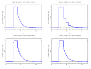
Optimal relaxed control determined by an indirect approach and by a direct approach on different control discretization grids.
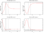
Differential states and corresponding adjoint variables in the indirect approach.
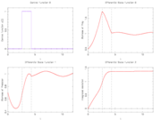
Control and differential states with only two switches.
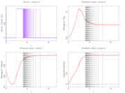
Control and differential states with 56 switches.


