Difference between revisions of "Lotka Volterra fishing problem (AMPL)"
(moved content from Lotka Volterra fishing problem page) |
(Replaced code with realistic values and implicit Euler) |
||
| Line 1: | Line 1: | ||
| + | This page contains a discretized version of the MIOCP [[Lotka Volterra fishing problem]] in [http://www.ampl.org AMPL] format. You should be aware of the comments regarding discretization made on the [[:Category:AMPL|AMPL overview]] page. | ||
=== AMPL === | === AMPL === | ||
| Line 5: | Line 6: | ||
<source lang="AMPL"> | <source lang="AMPL"> | ||
# ---------------------------------------------------------------- | # ---------------------------------------------------------------- | ||
| − | # Lotka Volterra fishing problem with collocation ( | + | # Lotka Volterra fishing problem with collocation (implicit Euler) |
# (c) Sebastian Sager | # (c) Sebastian Sager | ||
# ---------------------------------------------------------------- | # ---------------------------------------------------------------- | ||
| − | + | var x {I, 1..nx} >= 0; | |
| − | + | param c1 > 0; | |
| − | + | param c2 > 0; | |
| − | + | param ref1 > 0; | |
| − | + | ||
| − | param c1 | + | |
| − | param c2 | + | |
| − | param ref1 > 0; | + | |
param ref2 > 0; | param ref2 > 0; | ||
| − | |||
| − | |||
| − | |||
| − | |||
| − | |||
| − | |||
| − | |||
| − | |||
minimize Deviation: | minimize Deviation: | ||
| − | + | 0.5 * (dt[0]/ntperu) * ( (x[0,1]-ref1)^2 + (x[0,2]-ref2)^2 ) | |
| − | + | + 0.5 * (dt[nu-1]/ntperu) * ((x[nt,1]-ref1)^2 + (x[nt,2]-ref2)^2) | |
| − | + | + sum {i in I diff {0,nt} } ( (dt[uidx[i]]/ntperu) * | |
| − | + | ( (x[i,1] - ref1)^2 + (x[i,2] - ref2)^2 ) ) ; | |
subj to ODE_DISC_1 {i in I diff {0}}: | subj to ODE_DISC_1 {i in I diff {0}}: | ||
| − | + | x[i,1] = x[i-1,1] + (dt[uidx[i]]/ntperu) * | |
| + | ( x[i,1] - x[i,1]*x[i,2] - x[i,1]*c1*w[uidx[i]] ); | ||
subj to ODE_DISC_2 {i in I diff {0}}: | subj to ODE_DISC_2 {i in I diff {0}}: | ||
| − | + | x[i,2] = x[i-1,2] + (dt[uidx[i]]/ntperu) * | |
| + | ( - x[i,2] + x[i,1]*x[i,2] - x[i,2]*c2*w[uidx[i]] ); | ||
| + | |||
| + | subj to overall_stage_length: | ||
| + | sum {i in U} dt[i] = T; | ||
</source> | </source> | ||
a data file lotka_ampl.dat, | a data file lotka_ampl.dat, | ||
| Line 45: | Line 39: | ||
# Algorithmic parameters | # Algorithmic parameters | ||
| − | param ntperu := | + | param ntperu := 100; |
param nu := 100; | param nu := 100; | ||
| − | param nt := | + | param nt := 10000; |
| + | param nx := 2; | ||
| + | param fix_w := 0; | ||
| + | param fix_dt := 1; | ||
# Problem parameters | # Problem parameters | ||
param T := 12.0; | param T := 12.0; | ||
| − | param c1 := 0.4; | + | param c1 := 0.4; |
param c2 := 0.2; | param c2 := 0.2; | ||
| − | param ref1 := 1.0; | + | param ref1 := 1.0; |
param ref2 := 1.0; | param ref2 := 1.0; | ||
# Initial values differential states | # Initial values differential states | ||
| − | let x[0,1] := 0.5; | + | let x[0,1] := 0.5; let x[0,2] := 0.7; |
| − | let x[0,2] := 0.7; | + | fix x[0,1]; fix x[0,2]; |
| − | fix x[0,1]; | + | |
| − | fix x[0,2]; | + | |
# Initial values control | # Initial values control | ||
let {i in U} w[i] := 0.0; | let {i in U} w[i] := 0.0; | ||
| + | for {i in 0..(nu-1) / 2} { let w[i*2] := 1.0; } | ||
| + | let {i in U} dt[i] := T / nu; | ||
| − | |||
| − | |||
| − | |||
| − | |||
| − | |||
| − | |||
| − | |||
| − | |||
| − | |||
</source> | </source> | ||
and a running script lotka_ampl.run, | and a running script lotka_ampl.run, | ||
<source lang="AMPL"> | <source lang="AMPL"> | ||
| − | # | + | # ------------------------------------ |
| − | # Solve Lotka Volterra fishing problem | + | # Solve Lotka Volterra fishing problem |
| − | # | + | # ------------------------------------ |
| − | model | + | model ../general/ampl_general.mod; |
| − | data | + | model ampl_lotka_paper.mod; |
| + | data ampl_lotka_paper.dat; | ||
| + | data ../general/ampl_general.dat; | ||
| − | option solver | + | option presolve_eps 1e-10; |
| + | option solver ...; | ||
solve; | solve; | ||
| − | |||
| − | == | + | param myt; |
| + | let myt := 0; | ||
| + | for {i in I} { | ||
| + | if ( dt[uidx[i]] > 1e-6 ) then { | ||
| + | print myt, w[uidx[i]], x[i,1], x[i,2] > resultInt.txt; | ||
| + | } | ||
| + | let myt := myt + (dt[uidx[i]]/ntperu); | ||
| + | } | ||
| + | display w; | ||
| + | </source> | ||
| + | == Results == | ||
| − | + | The solution calculated by Bonmin (subversion revision number 1453, default settings, 3 GHz, Linux 2.6.28-13-generic, with ASL(20081205)) has an objective function value of <MATH>\Phi= 1.34434</MATH>, while the optimum of the relaxation is <MATH>\Phi=1.3423368</MATH>. Bonmin needs 35301 iterations and 2741 nodes (4899.97 seconds). Strong branching is done 81 times (1859 iterations), with 0 fathomed nodes and 0 fixed variables. The intervals on the equidistant grid on which <MATH>w(t) = 1</MATH> holds, counting from 0 to 99, are 20-32, 34, 36, 38, 40, 44, 53. | |
| − | + | ||
| − | The | + | |
| − | + | ||
| − | + | ||
| − | + | ||
| − | + | ||
| − | + | ||
| − | The | + | |
| − | + | ||
[[Category:AMPL]] | [[Category:AMPL]] | ||
Revision as of 17:14, 9 July 2009
This page contains a discretized version of the MIOCP Lotka Volterra fishing problem in AMPL format. You should be aware of the comments regarding discretization made on the AMPL overview page.
AMPL
The model in AMPL code for a fixed control discretization grid with a collocation method. We need a model file lotka_ampl.mod,
# ----------------------------------------------------------------
# Lotka Volterra fishing problem with collocation (implicit Euler)
# (c) Sebastian Sager
# ----------------------------------------------------------------
var x {I, 1..nx} >= 0;
param c1 > 0;
param c2 > 0;
param ref1 > 0;
param ref2 > 0;

minimize Deviation:
 0.5 * (dt[0]/ntperu) * ( (x[0,1]-ref1)^2 + (x[0,2]-ref2)^2 )
 + 0.5 * (dt[nu-1]/ntperu) * ((x[nt,1]-ref1)^2 + (x[nt,2]-ref2)^2)
 + sum {i in I diff {0,nt} } ( (dt[uidx[i]]/ntperu) *
   ( (x[i,1] - ref1)^2 + (x[i,2] - ref2)^2 ) ) ;

subj to ODE_DISC_1 {i in I diff {0}}:
 x[i,1] = x[i-1,1] + (dt[uidx[i]]/ntperu) *
  ( x[i,1] - x[i,1]*x[i,2] - x[i,1]*c1*w[uidx[i]] );

subj to ODE_DISC_2 {i in I diff {0}}:
 x[i,2] = x[i-1,2] + (dt[uidx[i]]/ntperu) *
  ( - x[i,2] + x[i,1]*x[i,2] - x[i,2]*c2*w[uidx[i]] );

subj to overall_stage_length:
 sum {i in U} dt[i] = T;
a data file lotka_ampl.dat,
# ------------------------------------
# Data: Lotka Volterra fishing problem
# ------------------------------------

# Algorithmic parameters
param ntperu := 100;
param nu := 100;
param nt := 10000;
param nx := 2;
param fix_w := 0;
param fix_dt := 1;

# Problem parameters
param T := 12.0;
param c1 := 0.4;
param c2 := 0.2;
param ref1 := 1.0;
param ref2 := 1.0;

# Initial values differential states
let x[0,1] := 0.5; let x[0,2] := 0.7;
fix x[0,1]; fix x[0,2];

# Initial values control
let {i in U} w[i] := 0.0;
for {i in 0..(nu-1) / 2} { let w[i*2] := 1.0; }
let {i in U} dt[i] := T / nu;
and a running script lotka_ampl.run,
# ------------------------------------
# Solve Lotka Volterra fishing problem
# ------------------------------------

model ../general/ampl_general.mod;
model ampl_lotka_paper.mod;
data ampl_lotka_paper.dat;
data ../general/ampl_general.dat;

option presolve_eps 1e-10;
option solver ...;

solve;

param myt;
let myt := 0;
for {i in I} {
	if ( dt[uidx[i]] > 1e-6 ) then {
		print myt, w[uidx[i]], x[i,1], x[i,2] > resultInt.txt;
	}
	let myt := myt + (dt[uidx[i]]/ntperu);
}

display w;
Results
The solution calculated by Bonmin (subversion revision number 1453, default settings, 3 GHz, Linux 2.6.28-13-generic, with ASL(20081205)) has an objective function value of 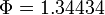 , while the optimum of the relaxation is
 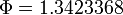 . Bonmin needs 35301 iterations and 2741 nodes (4899.97 seconds). Strong branching is done 81 times (1859 iterations), with 0 fathomed nodes and 0 fixed variables. The intervals on the equidistant grid on which
  holds, counting from 0 to 99, are 20-32, 34, 36, 38, 40, 44, 53.