Subway ride
| Subway ride | |
|---|---|
| State dimension: | 1 |
| Differential states: | 2 |
| Discrete control functions: | 1 |
| Interior point equalities: | 4 |
The subway ride optimal control problem goes back to work of <bibref>Bock1982</bibref> for the city of New York. In an extension, also velocity limits that lead to path-constrained arcs appear. The aim is to minimize the energy used for a subway ride from one station to another, taking into account boundary conditions and a restriction on the time.
Contents
Mathematical formulation
The MIOCP reads as
![\begin{array}{llcl}
\displaystyle \min_{x, w} & & & \int_{0}^{t_f} L(x, w) \; \mathrm{d} t \\[1.5ex]
\mbox{s.t.} & \dot{x}_0(t) & = & x_1(t), \\
& \dot{x}_1(t) & = & f_1(x,w), \\
& x(0) &=& (0, 0)^T, \\
& x(t_f) &=& (2112, 0)^T, \\
& w(t) &\in& \{1, 2, 3, 4\}, \quad t \in [0, t_f].
\end{array}](https://mintoc.de/images/math/4/a/6/4a6ee1811872c4cb4b583f0151f47167.png)
The terminal time  denotes the time of arrival of a subway train in the next station. The differential states
  and
and  describe position and velocity of the train, respectively. The train can be operated in one of four different modes,
  series,
  parallel,
  coasting, or
  braking that accelerate or decelerate the train and have different energy consumption.
Acceleration and energy comsumption are velocity-dependent. Hence, we will need switching functions 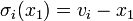 for given velocities
  .
.
The Lagrange term reads as
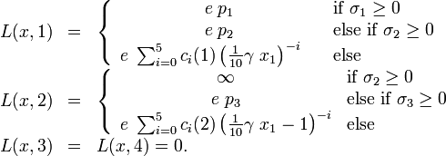
The right hand side function  reads as
The braking deceleration  can be varied between
  and a given
  . It can be shown that only maximal braking can be optimal, hence we fixed to without loss of generality.
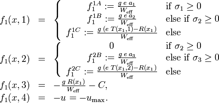
Occurring forces are
Details about the derivation of this model and the assumptions made can be found in <bibref>Bock1982</bibref> or in <bibref>Kraemer-Eis1985</bibref>.
Parameters
| Symbol | Value | Unit | Symbol | Value | Unit |
|---|---|---|---|---|---|
 |
78000 | lbs |  |
0.979474 | mph |
 |
85200 | lbs |  |
6.73211 | mph |
 |
2112 | ft |  |
14.2658 | mph |
 |
700 | ft |  |
22.0 | mph |
 |
1200 | ft |  |
24.0 | mph |
 |
 |
 |
 |
6017.611205 | lbs |
 |
100 | ft |
 |
12348.34865 | lbs |
 |
10 | - |  |
11124.63729 | lbs |
 |
0.045 | - | |
4.4 | ft / sec
|
 |
0.367 | - |  |
106.1951102 | - |
 |
32.2 |  |
 |
180.9758408 | - |
 |
1.0 | - |  |
354.136479 | - |
| Parameter | Value | Parameter | Value |
|---|---|---|---|
| b_0(1) | -0.1983670410E02 | c_0(1) | 0.3629738340E02 |
| b_1(1) | 0.1952738055E03 | c_1(1) | -0.2115281047E03 |
| b_2(1) | 0.2061789974E04 | c_2(1) | 0.7488955419E03 |
| b_3(1) | -0.7684409308E03 | c_3(1) | -0.9511076467E03 |
| b_4(1) | 0.2677869201E03 | c_4(1) | 0.5710015123E03 |
| b_5(1) | -0.3159629687E02 | c_5(1) | -0.1221306465E03 |
| b_0(2) | -0.1577169936E03 | c_0(2) | 0.4120568887E02 |
| b_1(2) | 0.3389010339E04 | c_1(2) | 0.3408049202E03 |
| b_2(2) | 0.6202054610E04 | c_1(2) | 0.3408049202E03 |
| b_3(2) | -0.4608734450E04 | c_3(2) | 0.8108316584E02 |
| b_4(2) | 0.2207757061E04 | c_4(2) | -0.5689703073E01 |
| b_5(2) | -0.3673344160E03 | c_5(2) | -0.2191905731E01 |
Reference Solutions
The optimal trajectory for this problem has been calculated by means of an indirect approach in <bibref>Bock1982</bibref><bibref>Kraemer-Eis1985</bibref>, and based on the direct multiple shooting method in <bibref>Sager2009</bibref>.
Variants
The given parameters have to be modified to match different parts of the track, subway train types, or amount of passengers. A minimization of travel time might also be considered.
The problem becomes more challenging, when additional point or path constraints are considered.
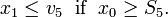
Point constraint
We consider the point constraint
for a given distance  and velocity
  . Note that the state is strictly monotonically increasing with time, as
  for all
  .
.
The optimal order of gears for  and
and  with the additional interior point constraints (\ref{FASOPOINTCON}) is
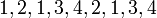 . The stage lengths between switches are 2.86362, 10.722, 15.3108, 5.81821, 1.18383, 2.72451, 12.917, 5.47402, and 7.98594
with
. The stage lengths between switches are 2.86362, 10.722, 15.3108, 5.81821, 1.18383, 2.72451, 12.917, 5.47402, and 7.98594
with  . For different parameters
  and we obtain the gear choice 1, 2, 1, 3, 2, 1, 3, 4 and stage lengths
2.98084, 6.28428, 11.0714, 4.77575, 6.0483, 18.6081, 6.4893, and 8.74202
with
and we obtain the gear choice 1, 2, 1, 3, 2, 1, 3, 4 and stage lengths
2.98084, 6.28428, 11.0714, 4.77575, 6.0483, 18.6081, 6.4893, and 8.74202
with 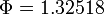 .
.
Path constraint
A more practical restriction are path constraints on subsets of the track. We will consider a problem with additional path constraints
The additional path constraint changes the qualitative behavior of the relaxed solution. While all solutions considered this far were bang-bang and the main work consisted in finding the switching points, we now have a path-constrained arc. The optimal solutions for refined grids yield a series of monotonically decreasing objective function values, where the limit is the best value that can be approximated by an integer feasible solution. In our case we obtain 1.33108, 1.31070, 1.31058, 1.31058, ...
Source Code
Model descriptions are available in
References
<bibreferences/>