Difference between revisions of "Time optimal car problem (GEKKO)"
From mintOC
(Create results page with Python GEKKO) |
m (Update with latest Gekko v1.0.5) |
||
| (One intermediate revision by the same user not shown) | |||
| Line 15: | Line 15: | ||
Z1 = m.Var(value=0, ub=330, lb=0) | Z1 = m.Var(value=0, ub=330, lb=0) | ||
Z2 = m.Var(value=0, ub=33, lb=0) | Z2 = m.Var(value=0, ub=33, lb=0) | ||
| − | m. | + | m.fix_final(Z2, 0) |
| − | m. | + | m.fix_final(Z1, 300) |
# set up the value we modify over the horizon | # set up the value we modify over the horizon | ||
| Line 60: | Line 60: | ||
== Results with APOPT (MINLP) == | == Results with APOPT (MINLP) == | ||
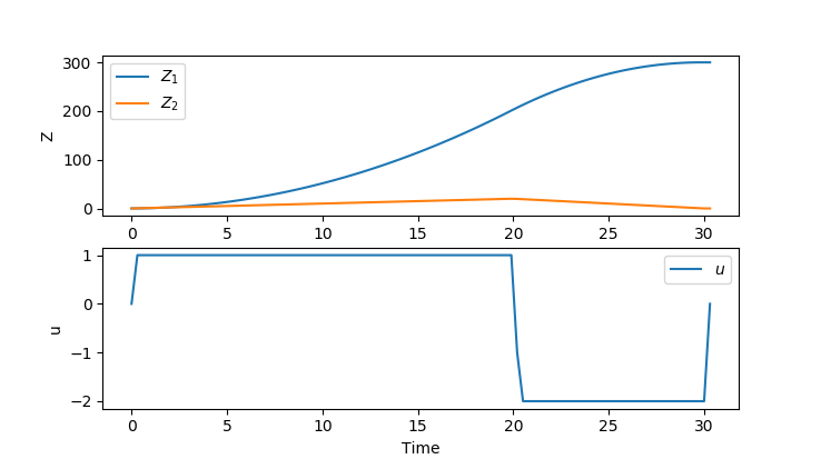
| − | An MINLP solution is calculated with APOPT with an objective function value of <math>30.3077</math>. | + | An MINLP solution is calculated with APOPT with an objective function value of <math>30.3077</math>. Thanks to [https://www.linkedin.com/in/tjasperson/ Tanner Jasperson] for providing a solution. |
[[File:Time_optimal_car_GEKKO.png]] | [[File:Time_optimal_car_GEKKO.png]] | ||
[[Category:Gekko]] | [[Category:Gekko]] | ||
Latest revision as of 14:23, 28 August 2022
This page contains a solution of the Time optimal car problem in GEKKO Python format. The GEKKO package is available with pip install gekko. The Python code uses orthogonal collocation and a simultaneous optimization method. The end point constraints are imposed as hard constraints.
from gekko import GEKKO
import matplotlib.pyplot as plt
import numpy as np

# set up the gekko model
m = GEKKO()

# set up the time (minimize the time with time scaling)
m.time = np.linspace(0, 1, 100)

# set up the variables
Z1 = m.Var(value=0, ub=330, lb=0)
Z2 = m.Var(value=0, ub=33, lb=0)
m.fix_final(Z2, 0)
m.fix_final(Z1, 300)

# set up the value we modify over the horizon
tf = m.FV(value=500, lb=0.1)
tf.STATUS = 1

# set up the MV
u = m.MV(integer=True, lb=-2, ub=1)
u.STATUS = 1

# set up the equations
m.Equation(Z1.dt() / tf == Z2)
m.Equation(Z2.dt() / tf == u)

# set the objective
m.Obj(tf)

# set up the options
m.options.IMODE = 6
m.options.SOLVER = 1

# solve
m.solve(disp=False)

# print the time
print("Total time taken: " + str(tf.NEWVAL))

# plot the results
plt.figure()
plt.subplot(211)
plt.plot(np.linspace(0,1,100)*tf.NEWVAL, Z1, label=r'$Z_1$')
plt.plot(np.linspace(0,1,100)*tf.NEWVAL, Z2, label=r'$Z_2$')
plt.ylabel('Z')
plt.legend()
plt.subplot(212)
plt.plot(np.linspace(0,1,100)*tf.NEWVAL, u, label=r'$u$')
plt.ylabel('u')
plt.xlabel('Time')
plt.legend()
plt.show()
Results with APOPT (MINLP)
An MINLP solution is calculated with APOPT with an objective function value of  . Thanks to Tanner Jasperson for providing a solution.
