Difference between revisions of "Urethane"
RobertLampel (Talk | contribs) (→Mathematical formulation) |
RobertLampel (Talk | contribs) (→Parameters) |
||
| (5 intermediate revisions by the same user not shown) | |||
| Line 21: | Line 21: | ||
</p> | </p> | ||
For ease of notation the chemical substances use the abbreviations | For ease of notation the chemical substances use the abbreviations | ||
| − | <table border="1"> | + | <table style="border-collapse:collapse;" border="1"> |
| − | <tr> | + | <tr style="border-bottom: 2pt solid black"> |
| − | <th>Letter</th> | + | <th style="border-right:2pt solid black; padding:2pt">Letter</th> |
| − | <th>Substance</th> | + | <th style="padding:2pt">Substance</th> |
</tr> | </tr> | ||
<tr> | <tr> | ||
| − | <td><math>A</math></td> | + | <td style="border-right:2pt solid black; text-align: center; padding:2pt"><math>A</math></td> |
| − | <td>Phenyl Isocyanate</td> | + | <td style="padding:2pt">Phenyl Isocyanate</td> |
</tr> | </tr> | ||
<tr> | <tr> | ||
| − | <td><math>B</math></td> | + | <td style="border-right:2pt solid black; text-align: center; padding:2pt"><math>B</math></td> |
| − | <td>Butanol</td> | + | <td style="padding:2pt">Butanol</td> |
</tr> | </tr> | ||
<tr> | <tr> | ||
| − | <td><math>C</math></td> | + | <td style="border-right:2pt solid black; text-align: center; padding:2pt"><math>C</math></td> |
| − | <td>Urethane <i>(Main Product)</i></td> | + | <td style="padding:2pt">Urethane <i>(Main Product)</i></td> |
</tr> | </tr> | ||
<tr> | <tr> | ||
| − | <td><math>D</math></td> | + | <td style="border-right:2pt solid black; text-align: center; padding:2pt"><math>D</math></td> |
| − | <td>Allophanate <i>(Secondary Product)</i></td> | + | <td style="padding:2pt">Allophanate <i>(Secondary Product)</i></td> |
</tr> | </tr> | ||
<tr> | <tr> | ||
| − | <td><math>E</math></td> | + | <td style="border-right:2pt solid black; text-align: center; padding:2pt"><math>E</math></td> |
| − | <td>Isocyanurate <i>(Byproduct)</i></td> | + | <td style="padding:2pt">Isocyanurate <i>(Byproduct)</i></td> |
</tr> | </tr> | ||
<tr> | <tr> | ||
| − | <td><math>L</math></td> | + | <td style="border-right:2pt solid black; text-align: center; padding:2pt"><math>L</math></td> |
| − | <td>Dimethyl Sulfoxide</td> | + | <td style="padding:2pt">Dimethyl Sulfoxide</td> |
</tr> | </tr> | ||
</table> | </table> | ||
| Line 105: | Line 105: | ||
</math> | </math> | ||
</p> | </p> | ||
| − | Each experiment lasts 80 | + | Each experiment lasts 80 hours. The beginning is Monday, 8 pm, the end Thursday, 4 pm. During the |
nights, the feed rates and the heating=cooling rate have to be zero due to safety rules. | nights, the feed rates and the heating=cooling rate have to be zero due to safety rules. | ||
Further control variables for experimental design are | Further control variables for experimental design are | ||
| Line 133: | Line 133: | ||
== Parameters == | == Parameters == | ||
| − | <table border="1.5"> | + | <table style="border-collapse:collapse" border="1.5"> |
<tr> | <tr> | ||
<td colspan=2 style="text-align: center; padding:5pt">Intial Values</td> | <td colspan=2 style="text-align: center; padding:5pt">Intial Values</td> | ||
| Line 170: | Line 170: | ||
| − | <table border="1.5"> | + | <table style="border-collapse:collapse" border="1.5"> |
<tr> | <tr> | ||
<td colspan=3 style="text-align: center; padding:5pt">Constants</td> | <td colspan=3 style="text-align: center; padding:5pt">Constants</td> | ||
| Line 211: | Line 211: | ||
== Optimal Experimental Design Problem == | == Optimal Experimental Design Problem == | ||
| − | <span style="color:red">To specify</span> | + | <!--<span style="color:red">To specify</span> |
In this approach, we add the so-called sensitivities <math>G=dy/d\theta</math>. For the differential equations this means | In this approach, we add the so-called sensitivities <math>G=dy/d\theta</math>. For the differential equations this means | ||
<p> | <p> | ||
| Line 218: | Line 218: | ||
</math> | </math> | ||
</p> | </p> | ||
| − | + | --> | |
Now we formulate the OED problem as described in [[#OEDUDE | [3]]]. | Now we formulate the OED problem as described in [[#OEDUDE | [3]]]. | ||
<p> | <p> | ||
Latest revision as of 10:07, 13 November 2024
| Urethane | |
|---|---|
| State dimension: | 1 |
| Differential states: | 11 |
| Discrete control functions: | 2 |
| Path constraints: | 4 |
| Interior point equalities: | 11 |
This page describes the Optimal Experimental Design Problem for the Urethane Reaction. The following formulation is taken from [1] and [2].
Contents
Chemical background
The reaction scheme of the urethane reaction is as follows:

For ease of notation the chemical substances use the abbreviations
| Letter | Substance |
|---|---|
 |
Phenyl Isocyanate |
 |
Butanol |
 |
Urethane (Main Product) |
 |
Allophanate (Secondary Product) |
 |
Isocyanurate (Byproduct) |
 |
Dimethyl Sulfoxide |
The reactor for the urethane reaction is a stirred tank and can be operated as a batch or semi-batch process with up to two feeds. In the reactor, phenyl isocyanate and butanol can be initially charged in the solvent dimethyl sulfoxide. In feed 1, phenyl isocyanate in dimethyl sulfoxide can be added, and in feed 2, butanol in dimethyl sulfoxide can be added. The internal temperature of the reactor is controllable.
Mathematical formulation
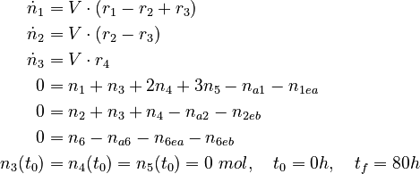
We can describe this process using a nonlinear DAE model

with

The molar numbers  of the species
  to
to  and
and  of the solvent
  are the state variables of the DAE system.
There are eight unknown parameters in this model:


 (for the reference temperature
  )
) of the reversible reaction
The two feeds are modelled by two monotonously increasing control functions
![\text{feed}_a,\text{feed}_b: \ [t_0,t_f] \rightarrow [0,1]](https://mintoc.de/images/math/1/b/8/1b8534800634691944bd17daec1b10bf.png)
describing the profiles of the accumulated feeds. Multiplied with the initial molar numbers within the feed vessels, we get the feed molar numbers:

The third control function is the temperature profile
![T: [t_0,t_f] \rightarrow [293.16 \ K, \ 473.16 \ K]](https://mintoc.de/images/math/9/5/3/9530558cca3d00bba6ea5d58b4b64609.png)
Each experiment lasts 80 hours. The beginning is Monday, 8 pm, the end Thursday, 4 pm. During the nights, the feed rates and the heating=cooling rate have to be zero due to safety rules. Further control variables for experimental design are
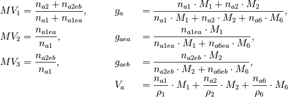
![MV_1 \in [0.1, 10], \ MV_2 \in [0, 1000]](https://mintoc.de/images/math/8/4/d/84d642bb2a5fa4d97c403d9a670b6c98.png) , and
, and ![MV_3 \in [0, 10]](https://mintoc.de/images/math/9/7/3/9730e32c3f23a9e86d44efc2510f4ed3.png)
![g_a \in [0, 0.8], \ g_{aea} \in [0, 0.9]](https://mintoc.de/images/math/b/7/a/b7aa0673ebf94e13850a6dcebde5c7b4.png) , and
, and ![g_{aeb} \in [0, 1]](https://mintoc.de/images/math/c/f/0/cf0bfa5a3b64a479b73da111ce671caa.png)
![V_a \in [0 m^3 , 0.00075 m^3 ]](https://mintoc.de/images/math/f/f/1/ff1e79de3f4ebe9005c130872eb7544c.png) of the species in the reactor.
of the species in the reactor.These quantities are connected to the initial molar numbers as follows

The remaining quantities are constants and shown in the parameter section. Three measurement methods are available:
In each experiment, 16 measurements can be selected out of 30 possible ones. We parametrize the time depending control functions using piecewise linear and continuous polynomials. Altogether we have 90 experimental design variables for each experiment: 7 control variables, 7 initial molar numbers, 30 weights on the measurements, and 46 variables due to the parametrization of the control functions.
Parameters
| Intial Values | |
 |
 |
 |
 |
 |
 |
 |
 |
 |
 |
 |
 |
 |
 |
| Constants | ||
| Molar Mass | Density | Reference Temperature |
|---|---|---|
 |
 |
 |
 |
 |
 |
 |
 |
 |
 |
 |
 |
 |
 |
molar gas constant  |
 |
 |
|
Optimal Experimental Design Problem
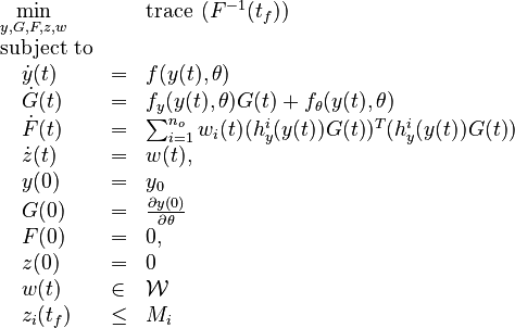
Now we formulate the OED problem as described in [3].

Here  is the observed function. The
evolution of the symmetric matrix
  is given by the weighted sum of observability Gramians
 for each observed function of states. The weights
  are the sampling decisions.
Miscellaneous and Further Reading
To be specified.
References
[1] "Numerische Methoden für Optimale Versuchsplanungsprobleme bei nichtlinearen DAE-Modellen " by S. Körkel
[2] "Numerical methods for optimum experimental design in DAE systems" by I. Bauer, H.G. Bock, S. Körkel and J.P. Schlöder
[3] "Optimal Experimental Design for Universal Differential Equations" by C. Plate, C.J. Martensen and S. Sager