Battery Storage

Battery Storage
State dimension:	1
Differential states:	1
Discrete control functions:	2

The battery storage problem models the optimal operation of a grid-scale battery energy storage system (BESS) over a 24-hour scheduling horizon. The operator minimises total electricity cost given a fixed, time-varying demand profile and a time-of-use electricity price signal. Both signals are piecewise-constant, stepping every four hours through six daily blocks. The two non-negative controls represent charging power and discharging power separately, which avoids the need for integer variables while keeping the physics transparent. The optimal strategy is to charge during cheap night-time periods and discharge during expensive morning and evening peak periods, yielding an energy-arbitrage policy.

Mathematical formulation

$\begin{array}{lll}\underset{P_c,P_d}{\min }& & \underset{0}{\overset{T}{\int }}p(t)(P_{\mathrm{l}\mathrm{o}\mathrm{a}\mathrm{d}}(t)-P_d(t)+P_c(t))\mathrm{d}t\\ \text{subject to}\\ \dot{x}(t)& =& \frac{{\eta }_c{P}_c(t)-P_d(t)/{\eta }_d}{E_{\mathrm{c}\mathrm{a}\mathrm{p}}},\\ x(0)& =& x_0,\\ x(T)& =& x_0,\\ x(t)& \in & [x_{\min },x_{\max }]\mathrm{\forall }t\in [0,T],\\ P_c(t)& \in & [0,P_{\max }]\mathrm{\forall }t\in [0,T],\\ P_d(t)& \in & [0,P_{\max }]\mathrm{\forall }t\in [0,T],\end{array}$

where $x(t)$ is the state of charge (SoC, dimensionless fraction of $E_{\mathrm{c}\mathrm{a}\mathrm{p}}$), $P_c(t)\ge 0$ is the charging power (kW), $P_d(t)\ge 0$ is the discharging power (kW), and $P_{\mathrm{g}\mathrm{r}\mathrm{i}\mathrm{d}}(t)=P_{\mathrm{l}\mathrm{o}\mathrm{a}\mathrm{d}}(t)-P_d(t)+P_c(t)$ is the net power drawn from the grid. The cyclic boundary condition $x(T)=x_0$ enforces a daily cycling constraint so the battery ends each day at the same charge level it started.

Price and demand profiles

Both $p(t)$ and $P_{\mathrm{l}\mathrm{o}\mathrm{a}\mathrm{d}}(t)$ are piecewise-constant step functions defined on six consecutive 4-hour blocks:

Block	Time interval (h)	$p(t)$ (€/kWh)	$P_{\mathrm{l}\mathrm{o}\mathrm{a}\mathrm{d}}(t)$ (kW)
1	[0, 4)	0.08	30
2	[4, 8)	0.20	60
3	[8, 12)	0.30	80
4	[12, 16)	0.15	50
5	[16, 20)	0.28	70
6	[20, 24]	0.10	35

The price pattern is cheap at night (blocks 1 and 6), expensive at the morning peak (block 3), and moderately expensive at the evening peak (block 5). The demand profile follows a corresponding load curve with low overnight consumption and a mid-morning peak.

Parameters

These fixed values are used within the model:

Symbol	Value	Description
$E_{\mathrm{c}\mathrm{a}\mathrm{p}}$	200 kWh	Battery energy capacity
$P_{\max }$	50 kW	Maximum charge / discharge power
${\eta }_c$	0.95	Charging efficiency
${\eta }_d$	0.95	Discharging efficiency
$x_{\min }$	0.10	Minimum state of charge
$x_{\max }$	0.90	Maximum state of charge
$x_0$	0.50	Initial (and final) state of charge
$T$	24 h	Scheduling horizon

Reference Solutions

Here is one local solution to the above control problem.

• Reference solution plots
• 
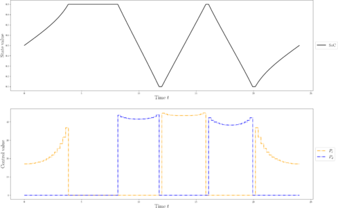  State of charge and optimal power schedule for a reference solution.

Miscellaneous and Further Reading

The battery storage optimal control problem arises in the operation of grid-scale energy storage, demand-response programs, and behind-the-meter storage systems. Formulating charging and discharging as two separate non-negative controls avoids the need for complementarity constraints or integer variables; the NLP relaxation is typically tight for cost profiles of this type because the optimizer has no incentive to charge and discharge simultaneously when round-trip efficiency is less than one. Numerical solutions generally exhibit a bang–bang structure in each control: the battery charges at full power during the cheapest blocks and discharges at full power during the most expensive blocks, with smooth transitions determined by the SoC bounds.

References

[1] Rahbar, N., Chai, C. C., & Zhang, R. (2015). Energy cooperation optimization in microgrids with renewable energy integration. IEEE Trans. Smart Grid, 6(3), 1482–1493.
[2] Nottrott, A., Kleissl, J., & Washom, B. (2013). Energy dispatch schedule optimization and cost benefit analysis for grid-connected, photovoltaic-battery storage systems. Renewable Energy, 55, 230–240.