Difference between revisions of "Diels-Alder Reaction Experimental Design"
| Line 255: | Line 255: | ||
\end{array} | \end{array} | ||
</math> | </math> | ||
| + | |||
| + | == Source Code == | ||
| + | |||
| + | * The VPLAN code using [[:Category: VPLAN | VPLAN code]] can be found in: [[Diels-Alder Reaction Experimental Design (VPLAN)]] | ||
== References == | == References == | ||
Revision as of 13:19, 1 February 2016
The Diels-Alder Reaction is an organic chemical reaction. A conjugated diene and a substituted alkene react and form a substituted cyclohexene system. Stefan Körkel used this model in his PhD thesis to compute optimum experimental designs.
Contents
Model Formulation
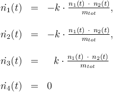
The reactionkinetics can be modelled by the following differential equation system:

The reaction velocity constant  consists of two parts. One part reflects the non-catalytic and the other the catalytic reaction. The velocity law follows the Arrhenius relation

Total mass:

Temperature in Kelvin:

The ODE system is summarized to:

Constraints
The control variables are constrained with respect to the mass of sample weights (initial mass):

and to the mass of active ingredient content (fraction of active substances):

Optimum Experimental Design Problem
The aim is to compute an optimal experimental design  which minimizes the uncertainties of the parameters
  . So, we have to solve the following optimum experimental design problem:
![\begin{array}{cll}
\displaystyle \min_{x,\ G,\ F,\ Tc,\ n_{a1},\ n_{a2},\ n_{a4},\ c_{kat},\ \vartheta(t)} && trace(F^{-1} (t_{end})) \\[1.5ex]
\mbox{s.t.} \\
\dot{x}(t) & = & f(x(t), u(t),p), \\
\\
h(t) & = & \frac{n_3(t) \ \cdot \ M_3}{m_{tot}} \ \cdot \ 100 \\
\\
\dot{G}(t) & = & f_x(x(t),u(t),p)G(t) \ + \ f_p(x(t),u(t),p) \\
\\
\dot{F}(t) & = & w(t) (h_x(x(t),u(t),p)G(t))^T (h_x(x(t),u(t),p)G(t)) \\
\\
0.1 & \le & n_{a1} \ \cdot \ M_1 \ + \ n_{a2} \ \cdot \ M_2 \ + \ n_{a4} \ \cdot \ M_4 \\
\\
10 & \ge & n_{a1} \ \cdot \ M_1 \ + \ n_{a2} \ \cdot \ M_2 \ + \ n_{a4} \ \cdot \ M_4 \\
\\
0.1 & \le & \frac{ n_{a1} \ \cdot \ M_1 \ + \ n_{a2} \ \cdot \ M_2 }{ n_{a1} \ \cdot \ M_1 \ + \ n_{a2} \ \cdot \ M_2 \ + \ n_{a4} \ \cdot \ M_4 } \\
\\
0.7 & \ge & \frac{ n_{a1} \ \cdot \ M_1 \ + \ n_{a2} \ \cdot \ M_2 }{ n_{a1} \ \cdot \ M_1 \ + \ n_{a2} \ \cdot \ M_2 \ + \ n_{a4} \ \cdot \ M_4 } \\
\\
\vartheta(t) & = & \left\{ \begin{array}{cl} \vartheta_{lo} + 273 & t \in [t_0,2] \\
\vartheta_{lo} + \frac{t-2}{6} ( \vartheta_{up} - \vartheta_{lo} ) + 273 & t \in [2,8] \\
\vartheta_{up} + 273 & t \in [8,t_{end}]
\end{array} \right. \\
& & x \in \mathcal{X},\,u \in \mathcal{U},\, p \in P .
\end{array}](https://mintoc.de/images/math/4/5/e/45ee8343b46c0bbfbc29bd4bef73b0a7.png)
| Name | Symbol | Initial value ( ) )
|
| Molar number 1 | 
|

|
| Molar number 2 | 
|

|
| Molar number 3 | 
|

|
| Solvent | 
|

|
| Name | Symbol | Value |
| Molar Mass | 
|
0.1362 |
| Molar Mass | 
|
0.09806 |
| Molar Mass | 
|
0.23426 |
| Molar Mass | 
|
0.236 |
| Universal gas constant | 
|
8.314 |
| Reference temperature | 
|
293 |
| St.dev of measurement error | 
|
1 |
Remember, in an optimum experimental design problem the parameters of the model are fixed. But, we minimize the parameter's uncertainties by optimizing over the control variables and functions.
| Name | Symbol | Value |
| Steric factor | 
|

|
| Steric factor | 
|

|
| Activation energie | 
|

|
| Activation energie | 
|

|
| Catalyst deactivation coefficient | 
|

|
with 
| Name | Symbol | Interval |
| Initial molar number 1 | 
|
[0.4,9.0] |
| Initial molar number 2 | 
|
[0.4,9.0] |
| Initial molar number 4 | 
|
[0.4,9.0] |
| Concentration of the catalyst | 
|
[0.0,6.0] |
| Name | Symbol | Time interval | Value interval | Initial value |
| Initial molar number 1 | 
|
![[t_0,2]](https://mintoc.de/images/math/2/c/c/2ccc6e33468338286f8ffb1f62564d08.png)
|
[20.0,100.0] | 20.0 |
| Initial molar number 1 | 
|
![[2,8]](https://mintoc.de/images/math/6/0/f/60fe7d62d10c721e8bc3c5e121a4f922.png)
|
[20.0,100.0] | 20.0 |
| Initial molar number 1 | 
|
![[8,t_{end}]](https://mintoc.de/images/math/c/7/8/c78ee1d499d759d6a276790fc2948860.png)
|
[20.0,100.0] | 20.0 |
Measurement grid

Source Code
- The VPLAN code using VPLAN code can be found in: Diels-Alder Reaction Experimental Design (VPLAN)
References
R. T. Morrison and R.N. Boyd. Organic Chemistry. Allyn and Bacon, Inc., 4th edition, 1983
S. Körkel. Numerische Methoden für Optimale Versuchsplanungsprobleme bei nichtlinearen DAE-Modellen.PhD thesis, Universität Heidelberg, Heidelber,2002