Difference between revisions of "Control of Heat Equation with Actuator Placement"
FelixMueller (Talk | contribs) (→Parameters) |
FelixMueller (Talk | contribs) (→Parameters) |
||
| Line 51: | Line 51: | ||
The parameter <math> \kappa </math> describes the thermal dissipativity of the material in the domain <math> \Omega </math>, it may vary in space. | The parameter <math> \kappa </math> describes the thermal dissipativity of the material in the domain <math> \Omega </math>, it may vary in space. | ||
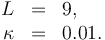
The parameter <math> L </math> indicates the number of possible actuator locations. They are distributed as indecated inthe picture. | The parameter <math> L </math> indicates the number of possible actuator locations. They are distributed as indecated inthe picture. | ||
| + | |||
| + | \begin{figure}[h] | ||
| + | \centering | ||
| + | \begin{tikzpicture} | ||
| + | \draw[step=1cm] (0,0) grid (8,4); | ||
| + | \filldraw[blue] (2,1) circle (4pt); | ||
| + | \filldraw[blue] (4,1) circle (4pt); | ||
| + | \filldraw[blue] (6,1) circle (4pt); | ||
| + | \filldraw[blue] (2,2) circle (4pt); | ||
| + | \filldraw[blue] (4,2) circle (4pt); | ||
| + | \filldraw[blue] (6,2) circle (4pt); | ||
| + | \filldraw[blue] (2,3) circle (4pt); | ||
| + | \filldraw[blue] (4,3) circle (4pt); | ||
| + | \filldraw[blue] (6,3) circle (4pt); | ||
| + | \end{tikzpicture} | ||
| + | \end{figure} | ||
==Reference solution== | ==Reference solution== | ||
Revision as of 17:39, 23 February 2016
| Control of Heat Equation with Actuator Placement | |
|---|---|
| State dimension: | 1 |
| Differential states: | 1 |
| Continuous control functions: |
 |
| Discrete control functions: |
|
| Path constraints: | 3 |
| Interior point equalities: | 2 |
This problem is governed by the heat equation and is adapted from Iftime and Demetriou ([Iftime2009]Author: Orest V. Iftime; Michael A. Demetriou
Journal: {A}utomatica
Number: 2
Pages: 312--323
Title: {O}ptimal control of switched distributed parameter systems with spatially scheduled actuators
Volume: 45
Year: 2009 ).
Its goal is to choose a place to apply an actuator in a given area depending on time.
We consider a rectangle
).
Its goal is to choose a place to apply an actuator in a given area depending on time.
We consider a rectangle ![\Omega=[0,1]\times[0,2]](https://mintoc.de/images/math/b/9/e/b9e9ecbd1ca99669f6d13a62bcf6142b.png) with the boundary
with the boundary  and the time horizon
 ![T=[0,10]](https://mintoc.de/images/math/0/a/e/0aef63dc3199780b7093eeb4bd8d74f5.png) as the domains.
The objective function is quadratic, its first term captures the desired final state
as the domains.
The objective function is quadratic, its first term captures the desired final state  , the second term regularize the state over time and the third term regularize the continuous controls.
The constraints are a source budget, which limits the quantity of placed actuators, and the two-dimensional heat equation with some source function.
Additionally, we assume Dirichlet boundary conditions and initial conditions.
, the second term regularize the state over time and the third term regularize the continuous controls.
The constraints are a source budget, which limits the quantity of placed actuators, and the two-dimensional heat equation with some source function.
Additionally, we assume Dirichlet boundary conditions and initial conditions.
Contents
[hide]Mathematical formulation
![\begin{array}{llcl}
\min\limits_{u,v,w}~~ &J(u,v)=||u(\cdot,\cdot,10)||_{2,\Omega}^2 +2||u(\cdot,\cdot,\cdot)||_{2,\Omega\times T}^2+\frac{1}{500}\sum\limits_{l=1}^L||v_l(\cdot)||^2_{2,T} & \\[10pt]
\text{ s.t.} ~~~~ &\frac{\partial u}{\partial t}(x,y,t)- \kappa \Delta u(x,y,t)=\sum\limits_{l=1}^9 v_l(t) f_l(x,y) &\text{ in }&\Omega\times T\\[10pt]
& u(x,y,t) =0 &\text{ on } &\partial\Omega\times T \\[10pt]
& u(x,y,0) = 100 \sin(\pi x)\sin(\pi y) &\text{ in }& \Omega\\[10pt]
& -M w_l(t)\leq v_l(t)\leq M w_l(t) \text{ for all } l\in \{1,\dots,L\} &\text{ in } & T \\[10pt]
& \sum\limits_{l=1}^L w_l(t) = 1 &\text{ in } & T\\[10pt]
& w_l(t)\in \{0,1\} \text{ for all } l\in \{1,\dots,L\} &\text{ in } &T.
\end{array}](https://mintoc.de/images/math/1/6/8/168b422f1c8bd993901de51eac922c9d.png)
Parameters
These fixed values are used within the model.
The parameter  describes the thermal dissipativity of the material in the domain
  , it may vary in space.
The parameter indicates the number of possible actuator locations. They are distributed as indecated inthe picture.
, it may vary in space.
The parameter indicates the number of possible actuator locations. They are distributed as indecated inthe picture.
\begin{figure}[h]
 \centering
 \begin{tikzpicture}
 \draw[step=1cm] (0,0) grid (8,4);
 \filldraw[blue] (2,1) circle (4pt);
 \filldraw[blue] (4,1) circle (4pt);
 \filldraw[blue] (6,1) circle (4pt);
 \filldraw[blue] (2,2) circle (4pt);
 \filldraw[blue] (4,2) circle (4pt);
 \filldraw[blue] (6,2) circle (4pt);
 \filldraw[blue] (2,3) circle (4pt);
 \filldraw[blue] (4,3) circle (4pt);
 \filldraw[blue] (6,3) circle (4pt);
  \end{tikzpicture}
\end{figure}
Reference solution
Source Code
References
| [Iftime2009] | Orest V. Iftime; Michael A. Demetriou (2009): {O}ptimal control of switched distributed parameter systems with spatially scheduled actuators . {A}utomatica, 45, 312--323 | |