Difference between revisions of "Diels-Alder Reaction Experimental Design"
(→Optimum Experimental Design Problem) |
(→Optimum Experimental Design Problem) |
||
| Line 72: | Line 72: | ||
The aim is to compute an optimal experimental design <math>\xi = (q,w)</math> which minimizes the uncertainties of the parameters <math>k_1, k_{cat}, E_1, E_{cat}, \lambda</math>. So, we have to solve the following optimum experimental design problem: | The aim is to compute an optimal experimental design <math>\xi = (q,w)</math> which minimizes the uncertainties of the parameters <math>k_1, k_{cat}, E_1, E_{cat}, \lambda</math>. So, we have to solve the following optimum experimental design problem: | ||
| − | + | ||
<math> | <math> | ||
\begin{array}{cll} | \begin{array}{cll} | ||
Revision as of 08:49, 9 December 2015
The Diels-Alder Reaction is an organic chemical reaction. A conjugated diene and a substituted alkene react and form a substituted cyclohexene system. Stefan Körkel used this model in his PhD thesis to compute optimum experimental designs.
Model Formulation
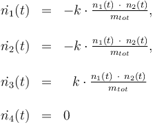
The reactionkinetics can be modelled by the following differential equation system:

The reaction velocity constant  consists of two parts. One part reflects the non-catalytic and the other the catalytic reaction. The velocity law follows the Arrhenius relation

Total mass:

Temperature in Kelvin:

The ODE system is summarized to:

Constraints
The control variables are constrained with respect to the mass of sample weights:

and to the mass of active ingredient content:

Optimum Experimental Design Problem
The aim is to compute an optimal experimental design  which minimizes the uncertainties of the parameters
  . So, we have to solve the following optimum experimental design problem:
![\begin{array}{cll}
\displaystyle \min_{x, G, F, Tc, n_{a1}} && trace(F^{-1} (t_{end})) \\[1.5ex]
\mbox{s.t.} \\
\dot{x}(t) & = & f(x(t), u(t),p), \\
\\
h(t) & = & \frac{n_3(t) \ \cdot \ M_3}{m_{tot}} \ \cdot \ 100 \\
\\
\dot{G}(t) & = & f_x(x(t),u(t),p)G(t) \ + \ f_p(x(t),u(t),p) \\
\\
\dot{F}(t) & = & w(t) (h_x(x(t),u(t),p)G(t))^T (h_x(x(t),u(t),p)G(t)) \\
\\
0.1 & \le & n_{a1} \ \cdot \ M_1 \ + \ n_{a2} \ \cdot \ M_2 \ + \ n_{a4} \ \cdot \ M_4 \\
\\
10 & \ge & n_{a1} \ \cdot \ M_1 \ + \ n_{a2} \ \cdot \ M_2 \ + \ n_{a4} \ \cdot \ M_4 \\
\\
0.1 & \le & \frac{ n_{a1} \ \cdot \ M_1 \ + \ n_{a2} \ \cdot \ M_2 }{ n_{a1} \ \cdot \ M_1 \ + \ n_{a2} \ \cdot \ M_2 \ + \ n_{a4} \ \cdot \ M_4 } \\
\\
0.7 & \ge & \frac{ n_{a1} \ \cdot \ M_1 \ + \ n_{a2} \ \cdot \ M_2 }{ n_{a1} \ \cdot \ M_1 \ + \ n_{a2} \ \cdot \ M_2 \ + \ n_{a4} \ \cdot \ M_4 } \\
\\
T(t) & = & \vartheta_{lo} + 273, \quad \forall \, t \in [t_0,2] \\
\\
T(t) & = & \vartheta_{lo} + \frac{t-2}{6} ( \vartheta_{up} - \vartheta_{lo} ) + 273 , \quad \forall \, t \in [2,8] \\
\\
T(t) & = & \vartheta_{up} + 273, \quad \forall \, t \in [8,t_{end}] \\
\\
x & \in & \mathcal{X},\,u \in \mathcal{U},\, p \in P.
\end{array}](https://mintoc.de/images/math/b/1/2/b12048d5672dcebe69377b610657f725.png)
| Name | Symbol | Initial value ( ) )
|
| Molar number 1 | 
|

|
| Molar number 2 | 
|

|
| Molar number 3 | 
|

|
| Solvent | 
|

|
| Name | Symbol | Value |
| Molar Mass | 
|
0.1362 |
| Molar Mass | 
|
0.09806 |
| Molar Mass | 
|
0.23426 |
| Molar Mass | 
|
0.236 |
| Universal gas constant | 
|
8.314 |
| Reference temperature | 
|
293 |
| St.dev of measurement error | 
|
1 |
| Name | Symbol | Value |
| Steric factor | 
|

|
| Steric factor | 
|

|
| Activation energie | 
|

|
| Activation energie | 
|

|
| Catalyst deactivation coefficient | 
|

|
with 
| Name | Symbol | Interval |
| Initial molar number 1 | 
|
[0.4,9.0] |
| Initial molar number 2 | 
|
[0.4,9.0] |
| Initial molar number 4 | 
|
[0.4,9.0] |
| Concentration of the catalyst | 
|
[0.0,6.0] |
| Name | Symbol | Time interval | Value interval | Initial value |
| Initial molar number 1 | 
|
[math>\t_{0}</math>,2] | [20.0,100.0] | 20.0 |
| Initial molar number 1 | 
|
[2,8] | [20.0,100.0] | 20.0 |
| Initial molar number 1 | 
|
[8,math>\t_{end}</math>] | [20.0,100.0] | 20.0 |
Measurement grid

References
R. T. Morrison and R.N. Boyd. Organic Chemistry. Allyn and Bacon, Inc., 4th edition, 1983
S. Körkel. Numerische Methoden für Optimale Versuchsplanungsprobleme bei nichtlinearen DAE-Modellen.PhD thesis, Universität Heidelberg, Heidelber,2002