Difference between revisions of "Diels-Alder Reaction Experimental Design"
(→Optimum Experimental Design Problem) |
(→Optimum Experimental Design Problem) |
||
| Line 97: | Line 97: | ||
\vartheta(t) & = & \vartheta_{up} + 273, \quad \forall \, t \in [8,t_{end}] \\ | \vartheta(t) & = & \vartheta_{up} + 273, \quad \forall \, t \in [8,t_{end}] \\ | ||
\\ | \\ | ||
| + | \vartheta(t) & = & \begin{cases} | ||
| + | test \\ | ||
| + | test | ||
| + | \end{cases} | ||
| + | |||
& & x \in \mathcal{X},\,u \in \mathcal{U},\, p \in P . | & & x \in \mathcal{X},\,u \in \mathcal{U},\, p \in P . | ||
\end{array} | \end{array} | ||
Revision as of 09:04, 9 December 2015
The Diels-Alder Reaction is an organic chemical reaction. A conjugated diene and a substituted alkene react and form a substituted cyclohexene system. Stefan Körkel used this model in his PhD thesis to compute optimum experimental designs.
Model Formulation
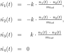
The reactionkinetics can be modelled by the following differential equation system:

The reaction velocity constant  consists of two parts. One part reflects the non-catalytic and the other the catalytic reaction. The velocity law follows the Arrhenius relation

Total mass:

Temperature in Kelvin:

The ODE system is summarized to:

Constraints
The control variables are constrained with respect to the mass of sample weights (initial mass):

and to the mass of active ingredient content (fraction of active substances):

Optimum Experimental Design Problem
The aim is to compute an optimal experimental design  which minimizes the uncertainties of the parameters
  . So, we have to solve the following optimum experimental design problem:
Failed to parse (PNG conversion failed; check for correct installation of latex and dvipng (or dvips + gs + convert)): {\begin{array}{cll}\displaystyle \min _{{x,\ G,\ F,\ Tc,\ n_{{a1}},\ n_{{a2}},\ n_{{a4}},\ c_{{kat}},\ \vartheta (t)}}&&trace(F^{{-1}}(t_{{end}}))\\[1.5ex]{\mbox{s.t.}}\\{\dot {x}}(t)&=&f(x(t),u(t),p),\\\\h(t)&=&{\frac {n_{3}(t)\ \cdot \ M_{3}}{m_{{tot}}}}\ \cdot \ 100\\\\{\dot {G}}(t)&=&f_{x}(x(t),u(t),p)G(t)\ +\ f_{p}(x(t),u(t),p)\\\\{\dot {F}}(t)&=&w(t)(h_{x}(x(t),u(t),p)G(t))^{T}(h_{x}(x(t),u(t),p)G(t))\\\\0.1&\leq &n_{{a1}}\ \cdot \ M_{1}\ +\ n_{{a2}}\ \cdot \ M_{2}\ +\ n_{{a4}}\ \cdot \ M_{4}\\\\10&\geq &n_{{a1}}\ \cdot \ M_{1}\ +\ n_{{a2}}\ \cdot \ M_{2}\ +\ n_{{a4}}\ \cdot \ M_{4}\\\\0.1&\leq &{\frac {n_{{a1}}\ \cdot \ M_{1}\ +\ n_{{a2}}\ \cdot \ M_{2}}{n_{{a1}}\ \cdot \ M_{1}\ +\ n_{{a2}}\ \cdot \ M_{2}\ +\ n_{{a4}}\ \cdot \ M_{4}}}\\\\0.7&\geq &{\frac {n_{{a1}}\ \cdot \ M_{1}\ +\ n_{{a2}}\ \cdot \ M_{2}}{n_{{a1}}\ \cdot \ M_{1}\ +\ n_{{a2}}\ \cdot \ M_{2}\ +\ n_{{a4}}\ \cdot \ M_{4}}}\\\\\vartheta (t)&=&\vartheta _{{lo}}+273,\quad \forall \,t\in [t_{0},2]\\\\\vartheta (t)&=&\vartheta _{{lo}}+{\frac {t-2}{6}}(\vartheta _{{up}}-\vartheta _{{lo}})+273,\quad \forall \,t\in [2,8]\\\\\vartheta (t)&=&\vartheta _{{up}}+273,\quad \forall \,t\in [8,t_{{end}}]\\\\\vartheta (t)&=&{\begin{cases}test\\test\end{cases}}&&x\in {\mathcal {X}},\,u\in {\mathcal {U}},\,p\in P.\end{array}}
| Name | Symbol | Initial value ( ) )
|
| Molar number 1 | 
|

|
| Molar number 2 | 
|

|
| Molar number 3 | 
|

|
| Solvent | 
|

|
| Name | Symbol | Value |
| Molar Mass | 
|
0.1362 |
| Molar Mass | 
|
0.09806 |
| Molar Mass | 
|
0.23426 |
| Molar Mass | 
|
0.236 |
| Universal gas constant | 
|
8.314 |
| Reference temperature | 
|
293 |
| St.dev of measurement error | 
|
1 |
Remember, in an optimum experimental design problem the parameters of the model are fixed. But, we minimize the parameter's uncertainties by optimizing over the control variables and functions.
| Name | Symbol | Value |
| Steric factor | 
|

|
| Steric factor | 
|

|
| Activation energie | 
|

|
| Activation energie | 
|

|
| Catalyst deactivation coefficient | 
|

|
with 
| Name | Symbol | Interval |
| Initial molar number 1 | 
|
[0.4,9.0] |
| Initial molar number 2 | 
|
[0.4,9.0] |
| Initial molar number 4 | 
|
[0.4,9.0] |
| Concentration of the catalyst | 
|
[0.0,6.0] |
| Name | Symbol | Time interval | Value interval | Initial value |
| Initial molar number 1 | 
|
![[t_0,2]](https://mintoc.de/images/math/2/c/c/2ccc6e33468338286f8ffb1f62564d08.png)
|
[20.0,100.0] | 20.0 |
| Initial molar number 1 | 
|
![[2,8]](https://mintoc.de/images/math/6/0/f/60fe7d62d10c721e8bc3c5e121a4f922.png)
|
[20.0,100.0] | 20.0 |
| Initial molar number 1 | 
|
![[8,t_{end}]](https://mintoc.de/images/math/c/7/8/c78ee1d499d759d6a276790fc2948860.png)
|
[20.0,100.0] | 20.0 |
Measurement grid

References
R. T. Morrison and R.N. Boyd. Organic Chemistry. Allyn and Bacon, Inc., 4th edition, 1983
S. Körkel. Numerische Methoden für Optimale Versuchsplanungsprobleme bei nichtlinearen DAE-Modellen.PhD thesis, Universität Heidelberg, Heidelber,2002