Car testdrive (lane change manoeuvre)

Car testdrive (lane change manoeuvre)
State dimension:	1
Differential states:	7
Continuous control functions:	3
Discrete control functions:	1
Interior point equalities:	7

The mathematical equations form a small-scale ODE model.

Mathematical formulation

For $t \in [t_0, t_f]$ almost everywhere the mixed-integer optimal control problem is given by

$\begin{array}{llcl} \displaystyle \min_{x, w} & t_f \\[1.5ex] \mbox{s.t.} & \dot{x}(t) & = & f( x(t), u(t), \mu(t)), \\ & x(0) &=& x_0, \\ & \mu(t) &\in& \{1, 2, 3, 4, 5\}. \end{array}$

Parameters

These fixed values are used within the model.

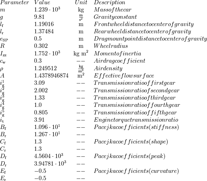
$\begin{array}{llcl} Parameter & Value & Unit & Description \\ m & 1.239\cdot 10^3 & \text{kg} & Mass of the car \\ g & 9.81 & \frac{\text{m}}{\text{s}^2} & Gravity constant \\ l_\text{f} & 1.19016 & \text{m} & Front wheel distance to center of gravity \\ l_\text{r} & 1.37484 & \text{m} & Rear wheel distance to center of gravity \\ e_\text{SP} & 0.5 & \text{m} & Drag mount point distance to center of gravity \\ R & 0.302 & \text{m} & Wheel radius \\ I_\text{zz} & 1.752\cdot 10^3 & \text{kg m}^2 & Moment of inertia \\ c_\text{w} & 0.3 & -- & Air drag coefficient \\ \rho & 1.249512 & \frac{\text{kg}}{\text{m}^3} & Air density \\ A & 1.4378946874 & \text{m}^2 & Effective flow surface \\ i^1_\text{g} & 3.09 & -- & Transmission ratio of first gear \\ i^2_\text{g} & 2.002 & -- & Transmission ratio of second gear \\ i^3_\text{g} & 1.33 & -- & Transmission ratio of third gear \\ i^4_\text{g} & 1.0 & -- & Transmission ratio of fourth gear \\ i^5_\text{g} & 0.805 & -- & Transmission ratio of fifth gear \\ i_\text{t} & 3.91 & -- & Engine torque transmission ratio \\ B_\text{f} & 1.096\cdot 10^1 & -- & Pacejka coefficients (stiffness) \\ B_\text{r} & 1.267\cdot 10^1 & -- & \\ C_\text{f} & 1.3 & -- & Pacejka coefficients (shape) \\ C_\text{r} & 1.3 & -- & \\ D_\text{f} & 4.5604\cdot 10^3 & -- & Pacejka coefficients (peak) \\ D_\text{r} & 3.94781\cdot 10^3 & -- & \\ E_\text{f} & -0.5 & -- & Pacejka coefficients (curvature) \\ E_\text{r} & -0.5 & -- & \\ \end{array}$

Test course

The double-lane change manoeuvre presented in <bibref>Gerdts2005</bibref> is realized by constraining the car's position onto a prescribed track at any time $t\in[t_0,t_\text{f}]$. Starting in the left position with an initial prescribed velocity, the driver is asked to manage a change of lanes modeled by an offset of 3.5 meters in the track. Afterwards he is asked to return to the starting lane. This manoeuvre can be regarded as an overtaking move or as an evasive action taken to avoid hitting an obstacle suddenly appearing on the starting lane.

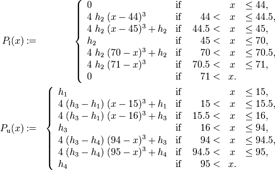
From a mathematical point of view, the test track is described by setting up piecewise cubic spline functions $P_\text{l}(x)$ and $P_\text{r}(x)$ modeling the top and bottom track boundary, given a horizontal position $x$.

$\begin{align} P_\text{l}(x) &:=& \left\{ \begin{array}{llrcl} 0 & \text{if } & & x & \leq 44, \\ 4\; h_2\; (x-44)^3 & \text{if } & 44 < & x & \leq 44.5, \\ 4\; h_2\; (x-45)^3 + h_2 & \text{if } & 44.5 < & x & \leq 45, \\ h_2 & \text{if } & 45 < & x & \leq 70, \\ 4\; h_2\; (70-x)^3 + h_2 & \text{if } & 70 < & x & \leq 70.5, \\ 4\; h_2\; (71-x)^3 & \text{if } & 70.5 < & x & \leq 71, \\ 0 & \text{if } & 71 < & x. & \\ \end{array} \right. \\ P_\text{u}(x) &:=& \left\{ \begin{array}{llrcl} h_1 & \text{if } & & x & \leq 15, \\ 4\; (h_3-h_1)\; (x-15)^3 + h_1 & \text{if } & 15 < & x & \leq 15.5, \\ 4\; (h_3-h_1)\; (x-16)^3 + h_3 & \text{if } & 15.5 < & x & \leq 16, \\ h_3 & \text{if } & 16 < & x & \leq 94, \\ 4\; (h_3-h_4)\; (94-x)^3 + h_3 & \text{if } & 94 < & x & \leq 94.5, \\ 4\; (h_3-h_4)\; (95-x)^3 + h_4 & \text{if } & 94.5 < & x & \leq 95, \\ h_4 & \text{if } & 95 < & x. & \\ \end{array} \right. \end{align}$

where $B=1.5\;\text{m}$ is the car's width and

$h_1 := 1.1\; B + 0.25, \quad h_2 := 3.5, \quad h_3 := 1.2\; B + 3.75,\quad h_4 := 1.3\; B + 0.25.$

Reference Solutions

Reference solutions for the case of a fixed time-grid are given in <bibref>Gerdts2005</bibref>. Solutions for a non-fixed time grid are given in <bibref>Gerdts2006</bibref>.

Variants

See testdrive overview page.

References

<bibreferences/>