Difference between revisions of "Bang-bang approximation of a traveling wave"
(Added reference solution) |
FelixMueller (Talk | contribs) |
||
| (8 intermediate revisions by 3 users not shown) | |||
| Line 1: | Line 1: | ||
| − | The following problem is an academic example of a PDE constrained optimal control problem with integer control constraints | + | {{Dimensions |
| − | + | |nd = 2 | |
| + | |nx = 1 | ||
| + | |nw = 1 | ||
| + | |nc = 2 | ||
| + | }} | ||
| + | |||
| + | The following problem is an academic example of a PDE constrained optimal control problem with integer control constraints | ||
| + | and was introduced in <bib id="Hante2009" />. | ||
The control task consists of choosing the boundary value of a transport equation from the extremal values of a traveling | The control task consists of choosing the boundary value of a transport equation from the extremal values of a traveling | ||
| Line 25: | Line 32: | ||
is the traveling wave (oscillating between 0 and 1), <math>c>0</math> is a (small) regularization parameter and | is the traveling wave (oscillating between 0 and 1), <math>c>0</math> is a (small) regularization parameter and | ||
| − | <math>\bigvee_0^1 q(t)\,dt</math> denotes the variation of q(\cdot) over the interval <math>[0,1]</math>. | + | <math>\bigvee_0^1 q(t)\,dt</math> denotes the variation of <math>q(\cdot)</math> over the interval <math>[0,1]</math>. |
Thereby, the solution of the transport equation has to be understood in the usual weak sense defined by the | Thereby, the solution of the transport equation has to be understood in the usual weak sense defined by the | ||
characteristic equations. | characteristic equations. | ||
| + | Systems biology | ||
| − | + | == Reference solution == | |
| − | == Reference | + | |
For <math>c=0.0075</math> the best known solution is given by | For <math>c=0.0075</math> the best known solution is given by | ||
| Line 39: | Line 46: | ||
where <math>\chi_{[a,b]}(t)</math> denotes the indicator function of the interval <math>[a,b]</math>. | where <math>\chi_{[a,b]}(t)</math> denotes the indicator function of the interval <math>[a,b]</math>. | ||
| + | |||
| + | <gallery caption="Obtained solution plots" widths="240px" heights="167px" perrow="3"> | ||
| + | Image:sinPGsws.png| Solution <math>q^*(t)</math> obtained using a projected gradient method based on switching time sensitivities. | ||
| + | Image:sinFinalTime.png| Corresponding plots of the differential states (blue) and the wave (red) at <math>t=1</math>. | ||
| + | </gallery> | ||
== References == | == References == | ||
| − | < | + | <biblist /> |
<!--List of all categories this page is part of. List characterization of solution behavior, model properties, ore presence of implementation details (e.g., AMPL for AMPL model) here --> | <!--List of all categories this page is part of. List characterization of solution behavior, model properties, ore presence of implementation details (e.g., AMPL for AMPL model) here --> | ||
| Line 48: | Line 60: | ||
[[Category:PDE model]] | [[Category:PDE model]] | ||
[[Category:Transport]] | [[Category:Transport]] | ||
| + | [[Category:Tracking objective]] | ||
Latest revision as of 17:02, 27 January 2016
| Bang-bang approximation of a traveling wave | |
|---|---|
| State dimension: | 2 |
| Differential states: | 1 |
| Discrete control functions: | 1 |
| Path constraints: | 2 |
The following problem is an academic example of a PDE constrained optimal control problem with integer control constraints
and was introduced in [Hante2009]Address: Berlin, Heidelberg
Author: Hante, Falk M.; Leugering, G\"unter
Booktitle: HSCC '09: Proceedings of the 12th International Conference on Hybrid Systems: Computation and Control
Pages: 209--222
Publisher: Springer-Verlag
Title: Optimal Boundary Control of Convention-Reaction Transport Systems with Binary Control Functions
Year: 2009 .
.
The control task consists of choosing the boundary value of a transport equation from the extremal values of a traveling
wave such that the  -distance between the traveling wave and the resulting flow is minimized.
Mathematical formulation
![\begin{array}{ll}
\displaystyle \min_{x, q} & \displaystyle \int_0^1\int_0^1 |x(t,s)-x_d(t,s)|^2\,ds\,dt + c \bigvee_0^1 q(t)\,dt \\[1.5ex]
\mbox{s.t.} & \displaystyle \frac{\partial}{\partial t}x(t,s)+\frac{\partial}{\partial s}x(t,s) = 0,\quad 0<s<1,~0<t<1\\[1.5ex]
& \displaystyle x(t,0) = q(t),\quad 0<t<1 \\
& \displaystyle x(0,s) = x_d(0,s),\quad 0<s<1 \\
& \displaystyle q(t) \in \{0,1\},\quad 0<t<1 \\
\end{array}](https://mintoc.de/images/math/9/5/a/95a039fa4651c9f229f07886c436bd8f.png)
where

is the traveling wave (oscillating between 0 and 1),  is a (small) regularization parameter and
 denotes the variation of
  over the interval
 ![[0,1]](https://mintoc.de/images/math/c/c/f/ccfcd347d0bf65dc77afe01a3306a96b.png) .
Thereby, the solution of the transport equation has to be understood in the usual weak sense defined by the
characteristic equations.
Systems biology
.
Thereby, the solution of the transport equation has to be understood in the usual weak sense defined by the
characteristic equations.
Systems biology
Reference solution
For  the best known solution is given by
![q^*(t)=\chi_{[0,0.2]}(t)+\chi_{[0.4,0.6]}(t)+\chi_{[0.8,1]}(t),\quad 0\leq t\leq 1](https://mintoc.de/images/math/a/5/d/a5de6b3b4df43206bf46ceaca874dea2.png)
where ![\chi_{[a,b]}(t)](https://mintoc.de/images/math/6/4/2/642109745edab961ba1c260274c7ea98.png) denotes the indicator function of the interval
denotes the indicator function of the interval ![[a,b]](https://mintoc.de/images/math/2/c/3/2c3d331bc98b44e71cb2aae9edadca7e.png) .
.
- Obtained solution plots
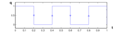
Solution
 obtained using a projected gradient method based on switching time sensitivities.
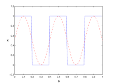
Corresponding plots of the differential states (blue) and the wave (red) at
 .
.


References
There were no citations found in the article.