Brachistochrone

Brachistochrone
State dimension:	1
Differential states:	3
Discrete control functions:	1

The brachistochrone problem (from Greek brachístos chrónos, "shortest time") is one of the founding problems of the calculus of variations, and serves as a classical benchmark in optimal control.

First posed by Johann Bernoulli in 1696 as a public challenge, the problem asks for the shape of a frictionless curve connecting two fixed points in a vertical plane such that a particle released from rest at the upper point reaches the lower point in minimum time under gravity. As an optimal control problem, the system state consists of the horizontal position, the downward vertical position, and the speed of the particle, while the control is the instantaneous angle of the velocity vector measured below the horizontal. The terminal time is free and is the quantity to be minimised; it is handled by augmenting it as a global time-scaling variable and optimising over a normalised unit horizon. The analytical solution is a cycloid, obtainable through Pontryagin's minimum principle or the classical Euler–Lagrange equations.

Mathematical formulation

$\begin{array}{lll}\underset{\theta ,t_{\mathrm{f}}}{\min }& & t_{\mathrm{f}}\\ \text{subject to}\\ \dot{x}(t)& =& v(t)\cos (\theta (t)),\\ \dot{y}(t)& =& v(t)\sin (\theta (t)),\\ \dot{v}(t)& =& g\sin (\theta (t)),\\ (x(0),y(0),v(0))& =& (0,0,0),\\ x(t_{\mathrm{f}})& =& x_{\mathrm{f}},\\ y(t_{\mathrm{f}})& =& y_{\mathrm{f}},\\ \theta (t)& \in & [0,\pi ]\mathrm{\forall }t\in [0,t_{\mathrm{f}}],\end{array}$

where $x(t)$ is the horizontal position (m), $y(t)$ is the downward vertical position (m, positive downward), and $v(t)$ is the speed of the particle (m/s). The control $\theta (t)\in [0,\pi ]$ is the angle of the velocity vector below the horizontal: $\theta =0$ corresponds to purely horizontal motion and $\theta =\pi /2$ to straight downward motion. The speed dynamics $\dot{v}=g\sin \theta$ follow from the component of gravitational acceleration along the direction of motion. Since $v(0)=0$, the particle starts from rest. The constraint $\theta \in [0,\pi ]$ restricts the particle to descent arcs (no upward motion).

Parameters

These fixed values are used within the model:

Symbol	Value	Description
$g$	9.81	Gravitational acceleration (m s−2)
$x_{\mathrm{f}}$	1.0	Target horizontal position (m)
$y_{\mathrm{f}}$	0.5	Target downward vertical position (m)

Reference Solutions

Here is one local solution to the above control problem.

• Reference solution plots
• 
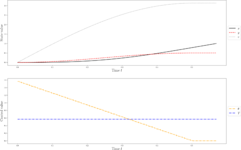  Optimal trajectory and control for the brachistochrone problem (cycloid solution).

Miscellaneous and Further Reading

The analytical solution is a cycloid: the locus traced by a point on the rim of a circle rolling along a flat surface. It can be parametrised as $x(\varphi )=r(\varphi -\sin \varphi )$, $y(\varphi )=r(1-\cos \varphi )$, where the radius $r$ is determined by the boundary conditions. The brachistochrone problem is a standard example in textbooks on optimal control and the calculus of variations, and is used as a test case for direct transcription methods due to its free terminal time and the mild singularity at $t=0$ where the speed vanishes. A detailed formulation and further discussion can be found in [1].

References

[1] Bryson, A. E., & Ho, Y.-C. (1975). Applied Optimal Control: Optimization, Estimation, and Control. Taylor & Francis.