Difference between revisions of "Lotka Volterra fishing problem"
(→Miscellaneous) |
|||
| Line 71: | Line 71: | ||
== Miscellaneous == | == Miscellaneous == | ||
| + | The Lotka Volterra fishing problem was introduced by Sebastian Sager in a proceedings paper <bibref>Sager2006</bibref> and reinvestigated in his PhD thesis <bibref>Sager2005</bibref>. These are also the references to look for more details. | ||
| + | |||
Testing Graphviz | Testing Graphviz | ||
| Line 77: | Line 79: | ||
</graphviz> | </graphviz> | ||
| − | + | == References == | |
| − | + | <bibreferences/> | |
| − | + | ||
| − | == | + | |
| − | + | ||
[[Category:ODE Model]] | [[Category:ODE Model]] | ||
Revision as of 20:34, 6 July 2008
This problem was set up as a simple benchmark problem. Despite of its simple structure, the optimal solution contains a singular arcs, making the Lotka Volterra fishing problem an ideal candidate for benchmarking of algorithms.
In this problem the Lotka Volterra equations for a predator-prey system have been augmented by an additional linear term, relating to fishing by man.
Model dimensions and properties
The model has the following dimensions:
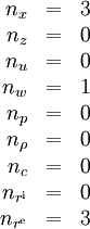
It is thus an ODE model with a single integer control function. The interior point equality conditions fix the initial values of the differential states.
Mathematical formulation
For ![t \in [t_0, t_f]](https://mintoc.de/images/math/5/5/8/55823791d9100bcb5461801aff4f6edd.png) the mixed-integer optimal control problem is given by
the mixed-integer optimal control problem is given by
![\begin{array}{llcl}
\displaystyle \min_{x, w} & x_2(t_f) \\[1.5ex]
\mbox{s.t.} & \dot{x}_0(t) & = & x_0(t) - x_0(t) x_1(t) - \; c_0 x_0(t) \; w(t), \\
& \dot{x}_1(t) & = & - x_1(t) + x_0(t) x_1(t) - \; c_1 x_1(t) \; w(t), \\
& \dot{x}_2(t) & = & (x_0(t) - 1)^2 + (x_1(t) - 1)^2, \\[1.5ex]
& x(0) &=& x_0, \\
& w(t) &\in& \{0, 1\}.
\end{array}](https://mintoc.de/images/math/e/9/3/e93178d5bd1af2eb33e434a69e6883c7.png)
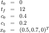
Initial values and parameters
Reference Solutions

Source Code
  double ref0 = 1, ref1 = 1;                 /* steady state with u == 0 */

  rhs[0] =   xd[0] - xd[0]*xd[1] - p[0]*u[0]*xd[0];
  rhs[1] = - xd[1] + xd[0]*xd[1] - p[1]*u[0]*xd[1];
  rhs[2] = (xd[0]-ref0)*(xd[0]-ref0) + (xd[1]-ref1)*(xd[1]-ref1);
Miscellaneous
The Lotka Volterra fishing problem was introduced by Sebastian Sager in a proceedings paper <bibref>Sager2006</bibref> and reinvestigated in his PhD thesis <bibref>Sager2005</bibref>. These are also the references to look for more details.
Testing Graphviz
<graphviz border='frame' format='svg'> digraph G {Hello->World!} </graphviz>
References
<bibreferences/>