Lotka Volterra fishing problem
| Lotka Volterra fishing problem | |
|---|---|
| State dimension: | 1 |
| Differential states: | 3 |
| Discrete control functions: | 1 |
| Interior point equalities: | 3 |
The Lotka Volterra fishing problem looks for an optimal fishing strategy to be performed on a fixed time horizon to bring the biomasses of both predator as prey fish to a prescribed steady state. The problem was set up as a small-scale benchmark problem. The well known Lotka Volterra equations for a predator-prey system have been augmented by an additional linear term, relating to fishing by man. The control can be regarded both in a relaxed, as in a discrete manner, corresponding to a part of the fleet, or the full fishing fleet.
It is thus an ODE model with a single integer control function. The interior point equality conditions fix the initial values of the differential states.
The optimal solution contains a singular arc, making the Lotka Volterra fishing problem an ideal candidate for benchmarking of algorithms.
Contents
Mathematical formulation
For ![t \in [t_0, t_f]](https://mintoc.de/images/math/5/5/8/55823791d9100bcb5461801aff4f6edd.png) almost everywhere the mixed-integer optimal control problem is given by
almost everywhere the mixed-integer optimal control problem is given by
![\begin{array}{llcl}
\displaystyle \min_{x, w} & x_2(t_f) \\[1.5ex]
\mbox{s.t.} & \dot{x}_0(t) & = & x_0(t) - x_0(t) x_1(t) - \; c_0 x_0(t) \; w(t), \\
& \dot{x}_1(t) & = & - x_1(t) + x_0(t) x_1(t) - \; c_1 x_1(t) \; w(t), \\
& \dot{x}_2(t) & = & (x_0(t) - 1)^2 + (x_1(t) - 1)^2, \\[1.5ex]
& x(0) &=& x_0, \\
& w(t) &\in& \{0, 1\}.
\end{array}](https://mintoc.de/images/math/e/9/3/e93178d5bd1af2eb33e434a69e6883c7.png)
Initial values and parameters
These fixed values are used within the model.
![\begin{array}{rcl}
[t_0, t_f] &=& [0, 12],\\
(c_0, c_1) &=& (0.4, 0.2),\\
x_0 &=& (0.5, 0.7, 0)^T.
\end{array}](https://mintoc.de/images/math/a/8/b/a8b6192b6bad3998ff2728a6397819b5.png)
Reference Solutions
If the problem is relaxed, i.e., we demand ![w(t) \in [0, 1]](https://mintoc.de/images/math/d/8/b/d8b966d03f416aecd2f9103830904e64.png) instead of
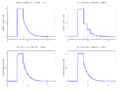
instead of 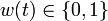 , the optimal solution can be determined by means of Pontryagins maximum principle. The optimal solution contains a singular arc, as can be seen in the plot of the optimal control. The two differential states and corresponding adjoint variables in the indirect approach are also displayed.
Optimal relaxed control determined by an indirect approach and by a direct approach on different control discretization grids.
Differential States and corresponding adjoint variables in the indirect approach.


Source Code
C
The differential equations in C code:
/* steady state with u == 0 */
double ref0 = 1, ref1 = 1;

/* Biomass of prey */
rhs[0] =   xd[0] - xd[0]*xd[1] - p[0]*u[0]*xd[0];
/* Biomass of predator */
rhs[1] = - xd[1] + xd[0]*xd[1] - p[1]*u[0]*xd[1];
/* Deviation from reference trajectory */
rhs[2] = (xd[0]-ref0)*(xd[0]-ref0) + (xd[1]-ref1)*(xd[1]-ref1);
AMPL
The model in AMPL code with a collocation method. We need a model file lotka_ampl.mod,
# ----------------------------------------------------------------
# Lotka Volterra fishing problem with collocation (explicit Euler)
# (c) Sebastian Sager
# ----------------------------------------------------------------

param T    > 0;
param nt   > 0;
param c1   > 0;
param c2   > 0;
param ref1 > 0;
param ref2 > 0;
param dt := T / (nt-1);
set I:= 0..nt;

var x {I, 1..2} >= 0;
var w {I} >= 0, <= 1 binary;

minimize Deviation:
	  0.5 * dt * ( (x[0,1] - ref1)*(x[0,1] - ref1) + (x[0,2] - ref2)*(x[0,2] - ref2) )
	+ 0.5 * dt * ( (x[nt,1] - ref1)*(x[nt,1] - ref1) + (x[nt,2] - ref2)*(x[nt,2] - ref2) )
	+ dt * sum {i in I diff {0,nt} } ( (x[i,1] - ref1)*(x[i,1] - ref1)
	                                 + (x[i,2] - ref2)*(x[i,2] - ref2) ) ;

subj to ODE_DISC_1 {i in I diff {0}}:
   x[i,1] = x[i-1,1] + dt * ( x[i-1,1] - x[i-1,1]*x[i-1,2] - x[i-1,1]*c1*w[i-1] );

subj to ODE_DISC_2 {i in I diff {0}}:
   x[i,2] = x[i-1,2] + dt * ( - x[i-1,2] + x[i-1,1]*x[i-1,2] - x[i-1,2]*c2*w[i-1] );
a data file lotka_ampl.dat,
# ------------------------------------
# Data: Lotka Volterra fishing problem
# ------------------------------------

# Algorithmic parameters
param nt := 100;

# Problem parameters
param T := 12.0;
param c1 := 0.4;
param c2 := 0.2;
param ref1 := 1.0;
param ref2 := 1.0;

# Initial values differential states
let x[0,1] := 0.5;
let x[0,2] := 0.7;
fix x[0,1];
fix x[0,2];

# Initial values control
let {i in I} w[i] := 0.0;
fix w[nt];

param mysum;
and a running script lotka_ampl.run,
# ----------------------------------------------------
# Solve Lotka Volterra fishing problem via collocation
# ----------------------------------------------------

model ampl_lotka.mod;
data ampl_lotka.dat;

option solver bonmin;

solve;
Miscellaneous and Further Reading
The Lotka Volterra fishing problem was introduced by Sebastian Sager in a proceedings paper <bibref>Sager2006</bibref> and revisited in his PhD thesis <bibref>Sager2005</bibref>. These are also the references to look for more details.
References
<bibreferences/>