Ramsey Growth

Ramsey Growth
State dimension:	1
Differential states:	1
Discrete control functions:	1

The Ramsey growth problem is a foundational benchmark in optimal control and macroeconomic theory.

First formulated by Frank Ramsey in 1928 [1] and later extended by Cass [2] and Koopmans [3], the Ramsey–Cass–Koopmans model determines the socially optimal path of capital accumulation and consumption for a representative household economy. The single state is the capital stock per effective worker, and the single control is consumption per effective worker. Capital accumulates through Cobb–Douglas production, net of depreciation, population growth, technological progress, and consumption. The objective is to maximise the present value of a stream of discounted CRRA utility over a finite horizon, plus a bequest value at the terminal time, which is equivalent to minimising its negative. The resulting optimal trajectories converge towards a steady-state balanced growth path.

Mathematical formulation

$\begin{array}{lll}\underset{c}{\min }& & -\underset{0}{\overset{T}{\int }}{e}^{-(\rho -n)t}\frac{c(t{)}^{1-\sigma }}{1-\sigma }\mathrm{d}t-V(k(T))\\ \text{subject to}\\ \dot{k}(t)& =& k(t{)}^{\alpha }-c(t)-(n+g+\delta )k(t),\\ k(0)& =& k_0,\\ k(t)& >& 0\mathrm{\forall }t\in [0,T],\\ c(t)& >& 0\mathrm{\forall }t\in [0,T],\end{array}$

where $k(t)$ is capital per effective worker, $c(t)$ is consumption per effective worker, $k^{\alpha }$ is the Cobb–Douglas production function (with total factor productivity normalised to one), and $c^{1-\sigma }/(1-\sigma )$ is the constant-relative-risk-aversion (CRRA) utility function. The effective discount rate in the objective is $\rho -n$, reflecting that utility is evaluated per capita while the economy grows at population rate $n$. As $\sigma \to 1$, the CRRA utility converges to $\ln c$ (logarithmic utility).

The terminal bequest value $V(k(T))$ approximates the discounted steady-state continuation:

$V(k(T))=e^{-(\rho -n)T}\frac{u(c_{\mathrm{s}\mathrm{s}}^{*})}{\rho -n}\min (\frac{k(T)}{k_{\mathrm{s}\mathrm{s}}^{*}},1),$

where $k_{\mathrm{s}\mathrm{s}}^{*}$ and $c_{\mathrm{s}\mathrm{s}}^{*}$ are the steady-state capital and consumption (see below).

Parameters

These fixed values are used within the model:

Symbol	Value	Description
$\alpha$	0.33	Capital share in production (Cobb–Douglas exponent)
$\delta$	0.05	Capital depreciation rate (year−1)
$n$	0.01	Population (labour) growth rate (year−1)
$g$	0.02	Technological progress rate (year−1)
$\rho$	0.04	Pure rate of time preference (year−1)
$\sigma$	1.5	Inverse of the intertemporal elasticity of substitution
$k_0$	3.0	Initial capital per effective worker
$T$	100	Planning horizon (years)

Reference Solutions

Here is one local solution to the above control problem.

• Reference solution plots
• 
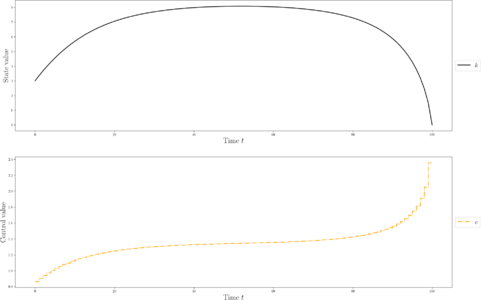  Optimal capital and consumption paths for a reference solution.

Miscellaneous and Further Reading

The steady-state capital stock satisfies the modified golden rule $\alpha (k_{\mathrm{s}\mathrm{s}}^{*}{)}^{\alpha -1}=\rho +\delta +n+g$, giving $k_{\mathrm{s}\mathrm{s}}^{*}=(\alpha /(\rho +\delta +n+g){)}^{1/(1-\alpha )}$ and $c_{\mathrm{s}\mathrm{s}}^{*}=(k_{\mathrm{s}\mathrm{s}}^{*}{)}^{\alpha }-(n+g+\delta )k_{\mathrm{s}\mathrm{s}}^{*}$. The optimal consumption path satisfies the Keynes–Ramsey rule $\dot{c}/c=(\alpha k^{\alpha -1}-\delta -\rho -g)/\sigma$. The problem is solved analytically in the infinite-horizon limit and numerically for finite horizons using shooting or direct methods; the finite-horizon version with a bequest value is a standard test for indirect shooting and continuation techniques.

References

[1] Ramsey, F. P. (1928). A mathematical theory of saving. The Economic Journal, 38(152), 543–559.
[2] Cass, D. (1965). Optimum growth in an aggregative model of capital accumulation. The Review of Economic Studies, 32(3), 233–240.
[3] Koopmans, T. C. (1965). On the concept of optimal economic growth. The Econometric Approach to Development Planning. North-Holland.