Category:GIOC
This category includes all generalized inverse optimal control problems.
To formalize this problem class, we define the following bilevel problem with differential states  , controls
  , model parameters
  , and convex multipliers
     subject to

                subject to
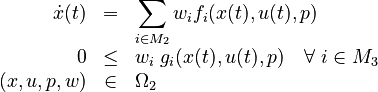
as a generalized inverse optimal control problem. Here  and
and  are properly defined function spaces. The variables
  indicate which objective functions, right hand side functions, and constraints are relevant in the inner problem. The variables are normalized for given index sets
  that partition the indices from
  to
to  . For normalization, we define the feasible set
 ![\mathcal{W} := \{ w \in [0,1]^{n_w}: \; \textstyle \sum^{i \in M_j} w_i = 1 \text{ for } j \in \{1,2,3\}\}](https://mintoc.de/images/math/4/f/8/4f8a91f62bf90121e2401d7f1384371a.png) . On the outer level, the feasible set is
. On the outer level, the feasible set is  , while on the inner level
  contains bounds, boundary conditions, mixed path and control constraints, and more involved constraints such as dwell time constraints. We have observational data
  , a measurement function
 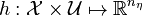 , a regularization function with a priori knowledge on parameters and weights
  and candidate functionals
 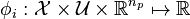 and functions
  and
and  for the unknown objective function, dynamics, and constraints, respectively. Two cases are of practical interest: first, the manual, often cumbersome and trial-and-error based a priori definition of all candidates
  by experts and second, a systematic, but often challenging automatic symbolic regression of these unknown functions.
On the outer level, a norm  and the regularization term
  define a data fit (regression) problem and relate to prior knowledge and statistical assumptions. On the inner level, the above bilevel problem is constrained by a possibly nonconvex optimal control problem. The unknown parts of this inner level optimal control problem are modeled as convex combinations of a finite set of candidates (and a multiplication of constraints
  with
with  that can be either zero or strictly positive). On the one hand the problem formulation is restrictive in the interest of a clearer presentation and might be further generalized, e.g., to multi-stage formulations involving differential-algebraic or partial differential equations. On the other hand, the problem class is quite generic and allows, e.g., the consideration of switched systems, periodic processes, different underlying function spaces and , and the usage of universal approximators such as neural networks as candidate functions.
Extensions
- The functions may also include integer controls.
- For some problems the functions may as well depend explicitely on the time
 .
. - The differential equations might depend on state-dependent switches.
- The variables may include boolean variables.
- The underlying process might be a multistage process.
- The dynamics might be unstable.
- There might be an underlying network topology.
- The integer control functions might have been (re)formulated by means of an outer convexification.
Note that a Lagrange term 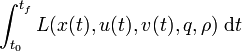 can be transformed into a Mayer-type objective functional.