Difference between revisions of "Control of Transmission Lines"
(Empty template for Control of Transmission Lines) |
|||
| (9 intermediate revisions by one other user not shown) | |||
| Line 1: | Line 1: | ||
| − | + | This problem was provided by Göttlich, Potschka, and Teuber <bib id="Goettlich2018" />. It is governed by a 2x2-system of conservation laws based on the telegraph equations for single transmission lines, which are then connected to form a network. The objective is to minimize the quadratic deviation of the load delivered to customer nodes from their demand by continuously controlling the power inflow to the network at the energy producer nodes and by discrete but time-varying switches at the coupling nodes inside the network. | |
== Mathematical formulation == | == Mathematical formulation == | ||
| + | |||
| + | The dynamics on the <math>r</math>-th transmission line with spatial variable <math>x \in [0, l_r]</math>, temporal variable <math>t \in [0, T]</math>, and state variable <math>\xi_r(x,t) = (\xi^+_r(x, t), \xi^-_r(x, t))</math> containing the characteristic variables for right-traveling and left-traveling components are given by the hyperbolic PDE system | ||
| + | <p> | ||
| + | <math> | ||
| + | \partial_t \xi_r(x,t) + \Lambda_r \xi_r(x,t) + B_r \xi_r(x,t) = 0, | ||
| + | </math> | ||
| + | </p> | ||
| + | with a diagonal 2x2-matrix <math>\Lambda_r</math> and a symmetric matrix <math>B_r</math>. We combine all <math>m</math> single line states to a large state vector <math>\boldsymbol{\xi}(x,t)</math> to obtain the system | ||
| + | <p> | ||
| + | <math> | ||
| + | \partial_t \boldsymbol{\xi} + \boldsymbol{\Lambda} \partial_x \boldsymbol{\xi} + \mathbf{B} \boldsymbol{\xi} = 0 | ||
| + | </math> | ||
| + | </p> | ||
| + | and formulate the coupling between the lines and the continuously controlled power inflow <math>\boldsymbol{u}(t)</math> as boundary conditions involving distribution matrices <math>\mathbf{D}^\pm(v)</math>, which depend on a discrete switching signal <math>\boldsymbol{v}(t)</math>, and constant matrices <math>\mathbf{\Lambda}^\pm</math> of size <math>m \times m</math> according to | ||
| + | <p> | ||
| + | <math> | ||
| + | \begin{pmatrix} | ||
| + | \boldsymbol{\Lambda}^+ & 0\\ | ||
| + | 0 & \mathbf{D}^-(\boldsymbol{v}(t)) | ||
| + | \end{pmatrix} \boldsymbol{\xi}(0,t) = | ||
| + | \begin{pmatrix} | ||
| + | \mathbf{D}^+(\boldsymbol{v}(t)) & 0\\ | ||
| + | 0 & \boldsymbol{\Lambda}^- | ||
| + | \end{pmatrix} \boldsymbol{\xi}(l,t) + | ||
| + | \begin{pmatrix} | ||
| + | \boldsymbol{\Lambda}^+ & 0\\ | ||
| + | 0 & 0 | ||
| + | \end{pmatrix} \boldsymbol{u}(t). | ||
| + | </math> | ||
| + | </p> | ||
| + | The continuous control <math>\boldsymbol{u}(t)</math> is subject to simple bounds. | ||
| + | |||
| + | The objective is to track the given demands <math>Q_s(t)</math> of consumers, which can be formulated as | ||
| + | <p> | ||
| + | <math> | ||
| + | \displaystyle \min_{\boldsymbol{v} \in \mathcal{V}, \boldsymbol{u} \in \mathcal{U}} \frac{1}{2}\sum_{s \in V_S} \int_0^{T} \left( Q_s(t) - \sum_{r \in \delta_{s}} \xi_r^+(l_r,t) \right)^2 dt, | ||
| + | </math> | ||
| + | </p> | ||
| + | where <math>V_S</math> is the set of consumer nodes and <math>\delta_s</math> is the set of all lines adjacent to vertex <math>s</math>. | ||
== Parameters == | == Parameters == | ||
| + | |||
| + | A detailed account of the network structures and parameter settings can be found in <bib id="Goettlich2018" /> and in the source code below. | ||
== Discretization == | == Discretization == | ||
| + | |||
| + | The mixed-integer variables <math>\boldsymbol{v}(t)</math> are transcribed via Partial Outer Convexification, i.e. the coupling conditions read | ||
| + | <p> | ||
| + | <math> | ||
| + | \begin{align} | ||
| + | \begin{pmatrix} | ||
| + | \boldsymbol{\Lambda}^+ & 0\\ | ||
| + | 0 & \sum_{c \in \Omega}\mathbf{D}_c^- b_c(t) | ||
| + | \end{pmatrix} \boldsymbol{\xi}(0,t) | ||
| + | &= | ||
| + | \begin{pmatrix} | ||
| + | \sum_{c \in \Omega} \mathbf{D}_c^+ b_c(t)) & 0\\ | ||
| + | 0 & \boldsymbol{\Lambda}^- | ||
| + | \end{pmatrix} \boldsymbol{\xi}(l,t) + | ||
| + | \begin{pmatrix} | ||
| + | \boldsymbol{\Lambda}^+ & 0\\ | ||
| + | 0 & 0 | ||
| + | \end{pmatrix} \boldsymbol{u}(t), \\ | ||
| + | \sum_{c \in \Omega} b_c(t) &= 1, \\ | ||
| + | b_c(t) &\in \{0,1\} \quad \forall c \in \Omega, | ||
| + | \end{align} | ||
| + | </math> | ||
| + | </p> | ||
| + | where each outer control <math>b_c(t)</math> contains the status of all switches and <math>\boldsymbol{D}_c^+, \boldsymbol{D}_c^-</math> are the constant distribution matrices for the configuration <math>c \in \Omega</math>. | ||
| + | |||
| + | The dynamics are discretized using Finite Volumes with upwind fluxes for the characteristic variables and explicit first-order time-stepping. | ||
== Reference Solution == | == Reference Solution == | ||
| + | |||
| + | We consider an extended tree network with 2 producers, 5 consumers and real-world demand data. | ||
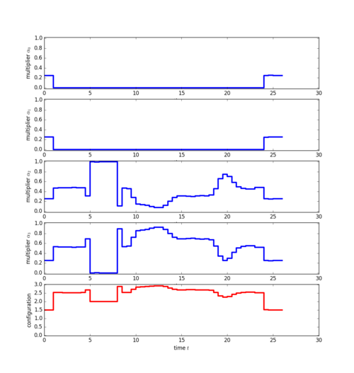
| + | After partial outer convexification (POC) and discretization, Ipopt delivers an NLP solution with objective value 2.804 and the following relaxed POC multipliers: | ||
| + | [[File:translines_relaxed_control.png|500px|Relaxed POC multipliers for switched controls]] | ||
| + | |||
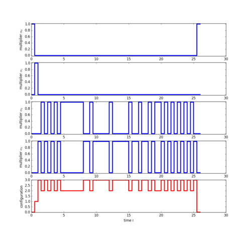
| + | Sum-Up Rounding with SOS1-constraint delivers the following integer feasible POC multipliers: | ||
| + | [[File:translines_switched_control.png|500px|POC multipliers for switched controls after Sum-Up-SOS1-Rounding]] | ||
| + | |||
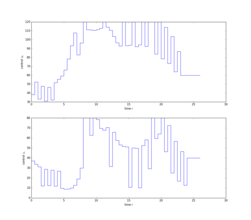
| + | Reoptimization with fixed Sum-Up Rounding decisions delivers an objective value of 3.152 and the following controls: | ||
| + | [[File:translines_cont_control.png|500px|Continuous controls]] | ||
| + | |||
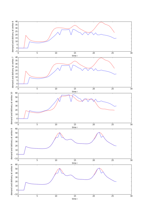
| + | The next figure compares the consumer demands (red) with the obtained power delivery (blue). | ||
| + | [[File:translines_demand_delivery.png|500px|Demand and delivery]] | ||
==Source Code== | ==Source Code== | ||
| + | |||
| + | The C++ code for the results in the paper is not publicly available, but a more user-friendly Python/CasADi-Version (without dwell-time constraints) is available on [https://github.com/apotschka/poc-transmission-lines GitHub/poc-transmission-lines]. A Python/Gurobi-Version (including dwell-time constraints) that solves the problem to global optimality is available on [https://github.com/jhelgert/pyTranslines GitHub/pyTranslines]. The latter also contains a specialized heuristic based on the CIAP decomposition in order to quickly find feasible solutions. | ||
==References== | ==References== | ||
| + | <biblist /> | ||
<!--List of all categories this page is part of. List characterization of solution behavior, model properties, ore presence of implementation details (e.g., AMPL for AMPL model) here --> | <!--List of all categories this page is part of. List characterization of solution behavior, model properties, ore presence of implementation details (e.g., AMPL for AMPL model) here --> | ||
Latest revision as of 08:07, 16 July 2021
This problem was provided by Göttlich, Potschka, and Teuber [Goettlich2018]Author: G{\"o}ttlich, Simone; Potschka, Andreas; Teuber, Claus
Institution: University of Mannheim
Note: Optimization Online 6312
Title: A partial outer convexification approach to control
transmission lines
Url: http://www.optimization-online.org/DB_HTML/2017/11/6312.html
Year: 2018 . It is governed by a 2x2-system of conservation laws based on the telegraph equations for single transmission lines, which are then connected to form a network. The objective is to minimize the quadratic deviation of the load delivered to customer nodes from their demand by continuously controlling the power inflow to the network at the energy producer nodes and by discrete but time-varying switches at the coupling nodes inside the network.
Contents
Mathematical formulation
The dynamics on the  -th transmission line with spatial variable
 ![x \in [0, l_r]](https://mintoc.de/images/math/e/f/d/efd5fa8c7741291758db47bbe865fd9c.png) , temporal variable
, temporal variable ![t \in [0, T]](https://mintoc.de/images/math/e/6/6/e66a2b7fedcba80ccb192b87440f8d9c.png) , and state variable
, and state variable  containing the characteristic variables for right-traveling and left-traveling components are given by the hyperbolic PDE system

with a diagonal 2x2-matrix  and a symmetric matrix
  . We combine all
  single line states to a large state vector
  to obtain the system

and formulate the coupling between the lines and the continuously controlled power inflow  as boundary conditions involving distribution matrices
  , which depend on a discrete switching signal
  , and constant matrices
  of size
  according to

The continuous control  is subject to simple bounds.
The objective is to track the given demands  of consumers, which can be formulated as

where  is the set of consumer nodes and
  is the set of all lines adjacent to vertex
  .
.
Parameters
A detailed account of the network structures and parameter settings can be found in [Goettlich2018]Author: G{\"o}ttlich, Simone; Potschka, Andreas; Teuber, Claus
Institution: University of Mannheim
Note: Optimization Online 6312
Title: A partial outer convexification approach to control
transmission lines
Url: http://www.optimization-online.org/DB_HTML/2017/11/6312.html
Year: 2018 and in the source code below.
Discretization
The mixed-integer variables  are transcribed via Partial Outer Convexification, i.e. the coupling conditions read

where each outer control  contains the status of all switches and
  are the constant distribution matrices for the configuration
  .
.
The dynamics are discretized using Finite Volumes with upwind fluxes for the characteristic variables and explicit first-order time-stepping.
Reference Solution
We consider an extended tree network with 2 producers, 5 consumers and real-world demand data.
After partial outer convexification (POC) and discretization, Ipopt delivers an NLP solution with objective value 2.804 and the following relaxed POC multipliers:

Sum-Up Rounding with SOS1-constraint delivers the following integer feasible POC multipliers:

Reoptimization with fixed Sum-Up Rounding decisions delivers an objective value of 3.152 and the following controls:

The next figure compares the consumer demands (red) with the obtained power delivery (blue).

Source Code
The C++ code for the results in the paper is not publicly available, but a more user-friendly Python/CasADi-Version (without dwell-time constraints) is available on GitHub/poc-transmission-lines. A Python/Gurobi-Version (including dwell-time constraints) that solves the problem to global optimality is available on GitHub/pyTranslines. The latter also contains a specialized heuristic based on the CIAP decomposition in order to quickly find feasible solutions.
References
There were no citations found in the article.