Difference between revisions of "DOW Experimental Design"
RobertLampel (Talk | contribs) (→Optimal Experimental Design Problem) |
RobertLampel (Talk | contribs) (→Parameters) |
||
| (53 intermediate revisions by 2 users not shown) | |||
| Line 7: | Line 7: | ||
}} | }} | ||
| − | The '''DOW Experimental Design problem''' models the OED problem for the parameter estimation problem formulated by the DOW Chemical Co. in 1981. The following formulation is taken from | + | The '''DOW Experimental Design problem''' models the OED problem for the parameter estimation problem formulated by the DOW Chemical Co. in 1981. The following formulation is taken from [[#Biegler1986|[1]]]. |
| − | + | ||
== Chemical background == | == Chemical background == | ||
| Line 31: | Line 30: | ||
MBMH \leftarrow K_1 \rightarrow MBM^- + H^+ \\ | MBMH \leftarrow K_1 \rightarrow MBM^- + H^+ \\ | ||
HA \leftarrow K_2 \rightarrow A^- + H^+ \\ | HA \leftarrow K_2 \rightarrow A^- + H^+ \\ | ||
| − | HABM \leftarrow | + | HABM \leftarrow K_3 \rightarrow ABM^- + H^+ |
\end{array} | \end{array} | ||
</math> | </math> | ||
| Line 41: | Line 40: | ||
<p> | <p> | ||
<math> | <math> | ||
| − | \begin{ | + | \begin{align} |
| − | \left[HBMH\right] = \left[ (MBMH)_N \right] + \left[ MBM^- \right] \\ | + | \left[HBMH\right] &= \left[ (MBMH)_N \right] + \left[ MBM^- \right] \\ |
| − | \left[HA\right] = \left[ (HA)_N \right] + \left[ A^- \right] \\ | + | \left[HA\right] &= \left[ (HA)_N \right] + \left[ A^- \right] \\ |
| − | \left[HABM\right] = \left[ (HABM)_N \right] + \left[ ABM^- \right] | + | \left[HABM\right] &= \left[ (HABM)_N \right] + \left[ ABM^- \right] |
| − | \end{ | + | \end{align} |
</math> | </math> | ||
</p> | </p> | ||
| − | Here <math>[ \ ]</math> denotes the concentration of the species in <math> | + | Here <math>[ \ ]</math> denotes the concentration of the species in <math>mol/kg</math>. |
By assuming the rapid acid-base reactions are at equilibrium, the equilibrium constants <math>K_1,K_2,K_3</math> can be defined as | By assuming the rapid acid-base reactions are at equilibrium, the equilibrium constants <math>K_1,K_2,K_3</math> can be defined as | ||
<p> | <p> | ||
<math> | <math> | ||
| − | \begin{ | + | \begin{align} |
| − | K_1 = \frac{[MBM^-][H^+]}{[(MBMH)_N]} \\ | + | K_1 &= \frac{[MBM^-][H^+]}{[(MBMH)_N]} \\ |
| − | + | K_2 &= \frac{[A^-][H^+]}{[(HA)_N]} \\ | |
| − | + | K_3 &= \frac{[ABM^-][H^+]}{[(HABM)_N]} | |
| − | \end{ | + | \end{align} |
</math> | </math> | ||
</p> | </p> | ||
| Line 63: | Line 62: | ||
<p> | <p> | ||
<math> | <math> | ||
| − | \begin{ | + | \begin{align} |
| − | \left[MBM^-\right] = \frac{K_1[MBMH]}{K_1 + [H^+]} & \quad (a) \\ | + | \left[MBM^-\right] &= \frac{K_1[MBMH]}{K_1 + [H^+]} && \quad (a) \\ |
| − | \left[A^-\right] = \frac{K_2[HA]}{K_2 + [H^+]} & \quad (b)\\ | + | \left[A^-\right] &= \frac{K_2[HA]}{K_2 + [H^+]} && \quad (b)\\ |
| − | \left[ABM^-\right] = \frac{K_3[HABM]}{K_3 + [H^+]}& \quad (c) | + | \left[ABM^-\right] &= \frac{K_3[HABM]}{K_3 + [H^+]} && \quad (c) |
| − | \end{ | + | \end{align} |
</math> | </math> | ||
</p> | </p> | ||
| Line 74: | Line 73: | ||
<p> | <p> | ||
<math> | <math> | ||
| − | \begin{ | + | \begin{align} |
| − | \frac{d[M^-]}{dt} = -k_1 \left[ M^- \right] \left[ BM \right] + k_{-1} \left[ MBM^- \right] - k_3 \left[ M^- \right]\left[ AB \right] + k_{-1} \left[ ABM^- \right] & \quad (d)\\ | + | \frac{d[M^-]}{dt} &= -k_1 \left[ M^- \right] \left[ BM \right] + k_{-1} \left[ MBM^- \right] - k_3 \left[ M^- \right]\left[ AB \right] + k_{-1} \left[ ABM^- \right] && \quad (d)\\ |
| − | \frac{d[BM]}{dt} = -k_1 \left[ M^- \right] \left[ BM \right] + k_{-1} \left[ MBM^- \right] - k_2 \left[ A^- \right]\left[ BM \right] & \quad (e)\\ | + | \frac{d[BM]}{dt} &= -k_1 \left[ M^- \right] \left[ BM \right] + k_{-1} \left[ MBM^- \right] - k_2 \left[ A^- \right]\left[ BM \right] && \quad (e)\\ |
| − | \frac{d[AB]}{dt} = -k_3 \left[ M^- \right] \left[ AB \right] + k_{-3} \left[ ABM^- \right] & \quad (f) | + | \frac{d[AB]}{dt} &= -k_3 \left[ M^- \right] \left[ AB \right] + k_{-3} \left[ ABM^- \right] && \quad (f) |
| − | \end{ | + | \end{align} |
</math> | </math> | ||
</p> | </p> | ||
| Line 85: | Line 84: | ||
<p> | <p> | ||
<math> | <math> | ||
| − | \begin{ | + | \begin{align} |
| − | \frac{d[MBMH]}{dt} = k_1 \left[ M^- \right] \left[ BM \right] | + | \frac{d[MBMH]}{dt} &= k_1 \left[ M^- \right] \left[ BM \right] - k_{-1} \left[ MBM^- \right] && \quad (g)\\ |
| − | \frac{d[HA]}{dt} = k_2 \left[ A^- \right] \left[ BM \right] & \quad (h)\\ | + | \frac{d[HA]}{dt} &= k_2 \left[ A^- \right] \left[ BM \right] && \quad (h)\\ |
| − | \frac{d[HABM]}{dt} = k_2 \left[ A^- \right] \left[ BM \right] + k_3 \left[ M^- \right] \left[ AB \right] - k_{-3} \left[ ABM^- \right]& \quad (i) | + | \frac{d[HABM]}{dt} &= k_2 \left[ A^- \right] \left[ BM \right] + k_3 \left[ M^- \right] \left[ AB \right] - k_{-3} \left[ ABM^- \right] && \quad (i) |
| − | \end{ | + | \end{align} |
</math> | </math> | ||
</p> | </p> | ||
| − | An electroneutrality constraint gives the hydrogen ion | + | An electroneutrality constraint gives the hydrogen ion concentration <math>\left[ H^+ \right]</math> as |
| − | + | ||
<p> | <p> | ||
<math> | <math> | ||
| Line 104: | Line 102: | ||
<math> k_3 = k_1, \quad k_{-3} = \frac{1}{2} k_{-1} </math> | <math> k_3 = k_1, \quad k_{-3} = \frac{1}{2} k_{-1} </math> | ||
</p> | </p> | ||
| − | With these assumptions, the three rate constants <math>k_1,k_2</math> and <math> | + | With these assumptions, the three rate constants <math>k_1,k_2</math> and <math>k_{-1}</math> must be estimated. Each of these can be fitted with two adjustable model parameters, assuming an Arrhenius temperature dependence. That is |
<p> | <p> | ||
<math> | <math> | ||
| Line 112: | Line 110: | ||
</math> | </math> | ||
</p> | </p> | ||
| − | Here <math>R</math> is the gas constant and <math>T</math> is reaction temperature in Kelvins. The | + | Here <math>R \approx 1.98720425864083 \ cal/(K \cdot mol) </math> is the gas constant and <math>T</math> is the reaction temperature in Kelvins. The parameters <math>\alpha_i</math>, given in <math>mol/( kg \cdot h)</math>, represent the pre-exponential factors and the <math>E_i</math>, with unit <math>cal/mol</math>, are the activation energies. |
== Mathematical formulation == | == Mathematical formulation == | ||
| Line 119: | Line 117: | ||
<p> | <p> | ||
<math> | <math> | ||
| − | \begin{ | + | \begin{align} |
| − | \dot{y}_1 = -k_2 y_8 y_2 & \quad (1),(h) \\ | + | \dot{y}_1 &= -k_2 y_8 y_2 && \quad (1),(h) \\ |
| − | \dot{y}_2 = -k_1 y_6 y_2 + k_{-1} y_{10} - k_2 y_8 y_2 & \quad (2),(e) \\ | + | \dot{y}_2 &= -k_1 y_6 y_2 + k_{-1} y_{10} - k_2 y_8 y_2 && \quad (2),(e) \\ |
| − | \dot{y}_3 = | + | \dot{y}_3 &= k_2 y_8 y_2 + k_1 y_6 y_4 - \frac{1}{2} k_{-1} y_9 && \quad (3),(i) \\ |
| − | \dot{y}_4 = -k_1 y_6 y_4 + \frac{1}{2} k_{-1} y_9 & \quad (4),(f) \\ | + | \dot{y}_4 &= -k_1 y_6 y_4 + \frac{1}{2} k_{-1} y_9 && \quad (4),(f) \\ |
| − | \dot{y}_5 = | + | \dot{y}_5 &= k_1 y_6 y_2 - k_{-1} y_{10} && \quad (5),(g) \\ |
| − | \dot{y}_6 = -k_1 (y_6 y_2 + y_6 y_4) + k_{-1} (y_{10} + \frac{1}{2} y_9) & \quad (6),(d) \\ | + | \dot{y}_6 &= -k_1 (y_6 y_2 + y_6 y_4) + k_{-1} (y_{10} + \frac{1}{2} y_9) && \quad (6),(d) \\ |
| − | y_7 = -\left[ Q^+ \right] + y_6 + y_8 + y_9 + y_{10} & \quad (7),(j)\\ | + | y_7 &= -\left[ Q^+ \right] + y_6 + y_8 + y_9 + y_{10} && \quad (7),(j)\\ |
| − | y_8 = \frac{\theta_8 y_1}{\theta_8 + y_7} & \quad (8),(b)\\ | + | y_8 &= \frac{\theta_8 y_1}{\theta_8 + y_7} && \quad (8),(b)\\ |
| − | y_9 = \frac{\theta_9 y_3}{\theta_9 + y_7} & \quad (9),(c)\\ | + | y_9 &= \frac{\theta_9 y_3}{\theta_9 + y_7} && \quad (9),(c)\\ |
| − | y_{10} = \frac{\theta_7 y_5}{\theta_7 + y_7} & \quad (10),(a) | + | y_{10} &= \frac{\theta_7 y_5}{\theta_7 + y_7} && \quad (10),(a) |
| − | \end{ | + | \end{align} |
</math> | </math> | ||
</p> | </p> | ||
| − | Here the letters in parentheses stand for the corresponding chemical process and the quantity <math>\left[Q^+\right]</math> is a constant during the reaction. | + | Here the letters in parentheses stand for the corresponding chemical process and the quantity <math>\left[Q^+\right]=0.0131</math> is a constant during the reaction. |
The nine parameters form the vector | The nine parameters form the vector | ||
<p> | <p> | ||
| Line 151: | Line 149: | ||
<p> | <p> | ||
<math> | <math> | ||
| − | \begin{ | + | \begin{align} |
| − | \dot{y}_7 = f_7 = f_6 + f_8 + f_9 + f_{10} & \quad (7') \\ | + | \dot{y}_7 &= f_7 = f_6 + f_8 + f_9 + f_{10} && \quad (7') \\ |
| − | \dot{y}_8 = f_8 = \frac{\theta_8 f_1 \cdot (\theta_8 + | + | \dot{y}_8 &= f_8 = \frac{\theta_8 f_1 \cdot (\theta_8 + y_7) - \theta_8 y_1 f_7}{(\theta_8 + y_7)^2} && \quad (8') \\ |
| − | \dot{y}_9 = f_9 = \frac{\theta_9 f_3 \cdot (\theta_9 + | + | \dot{y}_9 &= f_9 = \frac{\theta_9 f_3 \cdot (\theta_9 + y_7) - \theta_9 y_3 f_7}{(\theta_9 + y_7)^2} && \quad (9')\\ |
| − | \dot{y}_{10} = f_{10} = \frac{\theta_7 f_5 \cdot (\theta_7 + | + | \dot{y}_{10} &= f_{10} = \frac{\theta_7 f_5 \cdot (\theta_7 + y_7) - \theta_7 y_5 f_7}{(\theta_7 + y_7)^2} && \quad (10') |
| − | \end{ | + | \end{align} |
</math> | </math> | ||
</p> | </p> | ||
| Line 163: | Line 161: | ||
<p> | <p> | ||
<math> | <math> | ||
| − | \begin{ | + | \begin{align} |
| − | f_{y,m,n}(\cdot) = \frac{\partial f_m(\cdot)}{\partial y_n}, \quad m,n \in \{1,\ldots,10\} \\ | + | f_{y,m,n}(\cdot) &= \frac{\partial f_m(\cdot)}{\partial y_n}, \quad m,n \in \{1,\ldots,10\} \\ |
| − | f_{\theta,m,n}(\cdot) = \frac{\partial f_m(\cdot)}{\partial \theta_n}, \quad m \in \{1,\ldots,10\}; \ n\in \{1,\ldots,9\} | + | f_{\theta,m,n}(\cdot) &= \frac{\partial f_m(\cdot)}{\partial \theta_n}, \quad m \in \{1,\ldots,10\}; \ n\in \{1,\ldots,9\} |
| − | \end{ | + | \end{align} |
</math> | </math> | ||
| − | </p> | + | </p> |
== Parameters == | == Parameters == | ||
The initial parameter estimates are: | The initial parameter estimates are: | ||
| − | < | + | <table style="border-collapse: collapse;" border="1."> |
| − | + | <tr> | |
| − | + | <td style="text-align: center; padding:5pt"> <math> \alpha_1 </math> </td> | |
| − | + | <td style="text-align: center; padding:5pt"> <math>2.0 \cdot 10^{13} \ mol / (kg \cdot h)</math> </td> | |
| − | + | </tr> | |
| − | + | <tr> | |
| − | + | <td style="text-align: center; padding:5pt"><math>\alpha_2</math></td> | |
| − | + | <td style="text-align: center; padding:5pt"><math>2.0 \cdot 10^{13} \ mol / (kg \cdot h)</math></td> | |
| − | + | </tr> | |
| − | + | <tr> | |
| − | + | <td style="text-align: center; padding:5pt"><math>\alpha_{-1}</math></td> | |
| − | + | <td style="text-align: center; padding:5pt"><math>4.3 \cdot 10^{15} \ mol / (kg \cdot h)</math></td> | |
| − | + | </tr> | |
| − | + | <tr> | |
| − | </ | + | <td style="text-align: center; padding:5pt"><math>E_1</math></td> |
| + | <td style="text-align: center; padding:5pt"><math>2.0 \cdot 10^{4} \ cal / mol</math></td> | ||
| + | </tr> | ||
| + | <tr> | ||
| + | <td style="text-align: center; padding:5pt"><math>E_2</math></td> | ||
| + | <td style="text-align: center; padding:5pt"><math>2.0 \cdot 10^{4} \ cal / mol </math></td> | ||
| + | </tr> | ||
| + | <tr> | ||
| + | <td style="text-align: center; padding:5pt"><math>E_{-1}</math></td> | ||
| + | <td style="text-align: center; padding:5pt"><math>2.0 \cdot 10^{4} \ cal / mol</math></td> | ||
| + | </tr> | ||
| + | <tr> | ||
| + | <td style="text-align: center; padding:5pt"><math>K_1</math></td> | ||
| + | <td style="text-align: center; padding:5pt"><math>1.0\cdot 10^{-17} \ mol / kg</math></td> | ||
| + | </tr> | ||
| + | <tr> | ||
| + | <td style="text-align: center; padding:5pt"><math>K_2</math></td> | ||
| + | <td style="text-align: center; padding:5pt"><math>1.0\cdot 10^{-11} \ mol / kg</math></td> | ||
| + | </tr> | ||
| + | <tr> | ||
| + | <td style="text-align: center; padding:5pt"><math>K_3</math></td> | ||
| + | <td style="text-align: center; padding:5pt"><math>1.0\cdot 10^{-17} \ mol / kg</math></td> | ||
| + | </tr> | ||
| + | </table> | ||
| + | Note that for the calculations all temperatures given in <math>^{\circ}C</math> have to be rescaled to <math>K</math> by adding <math>273.15</math>. | ||
| + | |||
There are three datasets for different temperatures <math>T</math>, with corresponding starting values | There are three datasets for different temperatures <math>T</math>, with corresponding starting values | ||
| + | <table style="border-collapse: collapse;" border="1."> | ||
| + | <tr style="border-bottom: 2pt solid black;"> | ||
| + | <th style="border-right: 2pt solid black;"></th> | ||
| + | <th style="text-align: center; padding:5pt"> <math>40^\circ C </math></th> | ||
| + | <th style="text-align: center; padding:5pt"> <math>67^\circ C </math></th> | ||
| + | <th style="text-align: center; padding:5pt"> <math>100^\circ C </math></th> | ||
| + | </tr> | ||
| + | <tr> | ||
| + | <td style="text-align: center; padding:5pt; border-right: 2pt solid black;"> <math> y_1(0) </math> </td> | ||
| + | <td style="text-align: center; padding:5pt"> <math> 1.7066 </math> </td> | ||
| + | <td style="text-align: center; padding:5pt"> <math> 1.6749 </math> </td> | ||
| + | <td style="text-align: center; padding:5pt"> <math> 1.5608 </math> </td> | ||
| + | </tr> | ||
| + | <tr> | ||
| + | <td style="text-align: center; padding:5pt; border-right: 2pt solid black"><math>y_2(0)</math></td> | ||
| + | <td style="text-align: center; padding:5pt"><math>8.32</math></td> | ||
| + | <td style="text-align: center; padding:5pt"><math>8.2262</math></td> | ||
| + | <td style="text-align: center; padding:5pt"><math>8.3546</math></td> | ||
| + | </tr> | ||
| + | <tr> | ||
| + | <td style="text-align: center; padding:5pt; border-right: 2pt solid black"><math>y_3(0)</math></td> | ||
| + | <td style="text-align: center; padding:5pt"><math>0.01</math></td> | ||
| + | <td style="text-align: center; padding:5pt"><math>0.0104</math></td> | ||
| + | <td style="text-align: center; padding:5pt"><math>0.0082</math></td> | ||
| + | </tr> | ||
| + | <tr> | ||
| + | <td style="text-align: center; padding:5pt; border-right: 2pt solid black"><math>y_4(0)</math></td> | ||
| + | <td style="text-align: center; padding:5pt"><math>0</math></td> | ||
| + | <td style="text-align: center; padding:5pt"><math>0.0017</math></td> | ||
| + | <td style="text-align: center; padding:5pt"><math>0.0086</math></td> | ||
| + | </tr> | ||
| + | </table> | ||
| + | <!-- | ||
<p> | <p> | ||
<math> | <math> | ||
| Line 200: | Line 256: | ||
</math> | </math> | ||
</p> | </p> | ||
| + | --> | ||
The initial model conditions in addition to those given in the | The initial model conditions in addition to those given in the | ||
data sets are: | data sets are: | ||
| Line 206: | Line 263: | ||
\begin{array}{l} | \begin{array}{l} | ||
y_5 = 0 \\ | y_5 = 0 \\ | ||
| − | y_6 = | + | y_6 = [Q^+] \\ |
y_7 = \frac{1}{2} \cdot \left( -K_2 + \sqrt{K_2^2 + 4K_2 y_1(0)} \right) \\ | y_7 = \frac{1}{2} \cdot \left( -K_2 + \sqrt{K_2^2 + 4K_2 y_1(0)} \right) \\ | ||
y_8 = y_7 \\ | y_8 = y_7 \\ | ||
| Line 214: | Line 271: | ||
</math> | </math> | ||
</p> | </p> | ||
| + | |||
| + | To reduce the intercorrelation between the parameters in the rate constants, we apply the following reparametrization (cf. [[#Kristensen2004|[4]]].): | ||
| + | <p> | ||
| + | <math> | ||
| + | \begin{align} | ||
| + | k_i &= \alpha_i \cdot \exp \left( - \frac{E_i}{RT} \right) \\ | ||
| + | &= k_{0,i} \cdot \exp \left( - \frac{E_i}{R} \cdot \left( \frac{1}{T} - \frac{1}{T_0} \right) \right), \quad i=1,2,-1 | ||
| + | \end{align} | ||
| + | </math> | ||
| + | </p> | ||
| + | in which <math>k_{0,i} = \alpha_i \cdot \exp\left( - \frac{E_i}{RT_0} \right)</math>. The reference temperature in <math>T_0</math> is chosen as the average over all performed experiments, i.e., <math>T_0 = 69^\circ C</math>. Additionally, we add a logarithmic transformation, which gives rise to the following transformed starting values: | ||
| + | |||
| + | <table style="border-collapse: collapse;" border="1."> | ||
| + | <tr> | ||
| + | <td style="text-align: center; padding:5pt"> <math> \ln k_{0,1} </math> </td> | ||
| + | <td style="text-align: center; padding:5pt"> <math>1.194</math> </td> | ||
| + | </tr> | ||
| + | <tr> | ||
| + | <td style="text-align: center; padding:5pt"><math>\ln k_{0,2}</math></td> | ||
| + | <td style="text-align: center; padding:5pt"><math>1.194</math></td> | ||
| + | </tr> | ||
| + | <tr> | ||
| + | <td style="text-align: center; padding:5pt"><math>\ln k_{0,-1}</math></td> | ||
| + | <td style="text-align: center; padding:5pt"><math>6.565</math></td> | ||
| + | </tr> | ||
| + | <tr> | ||
| + | <td style="text-align: center; padding:5pt"><math>E_1</math></td> | ||
| + | <td style="text-align: center; padding:5pt"><math>2.0 \cdot 10^{4}</math></td> | ||
| + | </tr> | ||
| + | <tr> | ||
| + | <td style="text-align: center; padding:5pt"><math>E_2</math></td> | ||
| + | <td style="text-align: center; padding:5pt"><math>2.0 \cdot 10^{4} </math></td> | ||
| + | </tr> | ||
| + | <tr> | ||
| + | <td style="text-align: center; padding:5pt"><math>E_{-1}</math></td> | ||
| + | <td style="text-align: center; padding:5pt"><math>2.0 \cdot 10^{4}</math></td> | ||
| + | </tr> | ||
| + | <tr> | ||
| + | <td style="text-align: center; padding:5pt"><math>\ln K_1</math></td> | ||
| + | <td style="text-align: center; padding:5pt"><math>-34.54</math></td> | ||
| + | </tr> | ||
| + | <tr> | ||
| + | <td style="text-align: center; padding:5pt"><math>\ln K_2</math></td> | ||
| + | <td style="text-align: center; padding:5pt"><math>-25.33</math></td> | ||
| + | </tr> | ||
| + | <tr> | ||
| + | <td style="text-align: center; padding:5pt"><math>\ln K_3</math></td> | ||
| + | <td style="text-align: center; padding:5pt"><math>-39.14</math></td> | ||
| + | </tr> | ||
| + | </table> | ||
== Optimal Experimental Design Problem == | == Optimal Experimental Design Problem == | ||
| Line 222: | Line 329: | ||
<p> | <p> | ||
<math> | <math> | ||
| − | \begin{ | + | \begin{align} |
| − | k_{i,\alpha} := \frac{\partial k_i}{\partial \alpha_i} = \exp(-E_i/(RT)) \\ | + | k_{i,\alpha} &:= \frac{\partial k_i}{\partial \alpha_i} = \exp(-E_i/(RT)) \\ |
| − | k_{i,E} := \frac{\partial k_i}{\partial E_i} = -\frac{\alpha_i}{RT} \exp(-E_i/(RT)) | + | k_{i,E} &:= \frac{\partial k_i}{\partial E_i} = -\frac{\alpha_i}{RT} \exp(-E_i/(RT)) |
| − | \end{ | + | \end{align} |
</math> | </math> | ||
</p> | </p> | ||
| Line 262: | Line 369: | ||
<p> | <p> | ||
<math> | <math> | ||
| − | \begin{ | + | \begin{align} |
| − | f_y(\cdot) \in \mathbb{R}^{10 \times 10} \quad \text{ with } (f_y)_{i,j} = f_{y,i,j}, \\ | + | f_y(\cdot) &\in \mathbb{R}^{10 \times 10} \quad &&\text{ with } (f_y)_{i,j} = f_{y,i,j}, \\ |
| − | f_\theta(\cdot) \in \mathbb{R}^{10 \times 9} \quad \text{ with } (f_\theta)_{i,j} = | + | f_\theta(\cdot) &\in \mathbb{R}^{10 \times 9} \quad &&\text{ with } (f_\theta)_{i,j} = f_{\theta,i,j} |
| − | \end{ | + | \end{align} |
</math> | </math> | ||
</p> | </p> | ||
| Line 275: | Line 382: | ||
</p> | </p> | ||
| − | Now we formulate the OED problem as described in | + | Now we formulate the OED problem as described in [[#OEDUDE | [2]]]. |
<p> | <p> | ||
<math> | <math> | ||
| Line 305: | Line 412: | ||
== References == | == References == | ||
| − | + | <span id="Biegler1986">[1]</span> "Nonlinear Parameter Estimation: a Case Study Comparison" by L. T. Biegler and J. J. Damiano <br> | |
| − | < | + | <span id="OEDUDE">[2]</span> "Optimal Experimental Design for Universal Differential Equations" by C. Plate, C.J. Martensen and S. Sager <br> |
| − | < | + | <span id="Stortelder1998">[3]</span> "Parameter estimation in nonlinear systems" by W.J.H. Stortelder <br> |
| − | + | <span id="Kristensen2004">[4]</span> "Parameter Estimation in Nonlinear Dynamical Systems" by Morten Rode Kristensen <br> | |
<!--List of all categories this page is part of. List characterization of solution behavior, model properties, ore presence of implementation details (e.g., AMPL for AMPL model) here --> | <!--List of all categories this page is part of. List characterization of solution behavior, model properties, ore presence of implementation details (e.g., AMPL for AMPL model) here --> | ||
Latest revision as of 11:31, 18 February 2025
| DOW Experimental Design | |
|---|---|
| State dimension: | 1 |
| Differential states: | 11 |
| Discrete control functions: | 2 |
| Path constraints: | 4 |
| Interior point equalities: | 11 |
The DOW Experimental Design problem models the OED problem for the parameter estimation problem formulated by the DOW Chemical Co. in 1981. The following formulation is taken from [1].
Contents
Chemical background
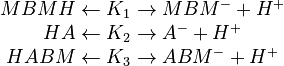
The chemical species are disguised for proprietary reasons and the desired reaction is given by  , where
  is the desired product. The reactions are described as follows:
Slow Kinetic Reactions:

Acid-Base Reactions:
In order to devise a model to account for these reactions, it is first necessary to distinguish between the overall concentration of a species and the concentration of its neutral form. Overall concentrations are defined for three components based on neutral and ionic species
![\begin{align}
\left[HBMH\right] &= \left[ (MBMH)_N \right] + \left[ MBM^- \right] \\
\left[HA\right] &= \left[ (HA)_N \right] + \left[ A^- \right] \\
\left[HABM\right] &= \left[ (HABM)_N \right] + \left[ ABM^- \right]
\end{align}](https://mintoc.de/images/math/8/a/9/8a90809e1d9fb52552b742b87f38a098.png)
Here ![[ \ ]](https://mintoc.de/images/math/7/5/4/7541b1af090dec7db3eb1953f2b90cc1.png) denotes the concentration of the species in
denotes the concentration of the species in  .
By assuming the rapid acid-base reactions are at equilibrium, the equilibrium constants
.
By assuming the rapid acid-base reactions are at equilibrium, the equilibrium constants  can be defined as
![\begin{align}
K_1 &= \frac{[MBM^-][H^+]}{[(MBMH)_N]} \\
K_2 &= \frac{[A^-][H^+]}{[(HA)_N]} \\
K_3 &= \frac{[ABM^-][H^+]}{[(HABM)_N]}
\end{align}](https://mintoc.de/images/math/0/f/c/0fc9353e835b909394feb2943063cf73.png)
The anionic species may then be represented by
![\begin{align}
\left[MBM^-\right] &= \frac{K_1[MBMH]}{K_1 + [H^+]} && \quad (a) \\
\left[A^-\right] &= \frac{K_2[HA]}{K_2 + [H^+]} && \quad (b)\\
\left[ABM^-\right] &= \frac{K_3[HABM]}{K_3 + [H^+]} && \quad (c)
\end{align}](https://mintoc.de/images/math/9/e/e/9ee28304dd2ce28499942f31c87106a4.png)
Material balance equations for the three reactants in the slow kinetic reactions yield:
![\begin{align}
\frac{d[M^-]}{dt} &= -k_1 \left[ M^- \right] \left[ BM \right] + k_{-1} \left[ MBM^- \right] - k_3 \left[ M^- \right]\left[ AB \right] + k_{-1} \left[ ABM^- \right] && \quad (d)\\
\frac{d[BM]}{dt} &= -k_1 \left[ M^- \right] \left[ BM \right] + k_{-1} \left[ MBM^- \right] - k_2 \left[ A^- \right]\left[ BM \right] && \quad (e)\\
\frac{d[AB]}{dt} &= -k_3 \left[ M^- \right] \left[ AB \right] + k_{-3} \left[ ABM^- \right] && \quad (f)
\end{align}](https://mintoc.de/images/math/6/e/7/6e7496978a48089559abb74f5d4859ac.png)
From stoichiometry, rate expressions can also be written for the total species:
![\begin{align}
\frac{d[MBMH]}{dt} &= k_1 \left[ M^- \right] \left[ BM \right] - k_{-1} \left[ MBM^- \right] && \quad (g)\\
\frac{d[HA]}{dt} &= k_2 \left[ A^- \right] \left[ BM \right] && \quad (h)\\
\frac{d[HABM]}{dt} &= k_2 \left[ A^- \right] \left[ BM \right] + k_3 \left[ M^- \right] \left[ AB \right] - k_{-3} \left[ ABM^- \right] && \quad (i)
\end{align}](https://mintoc.de/images/math/f/b/a/fbaa5e23b96608be8ee90fc5f138b1af.png)
An electroneutrality constraint gives the hydrogen ion concentration ![\left[ H^+ \right]](https://mintoc.de/images/math/a/d/0/ad0539982a2a429c51ee7e34fc22d0d4.png) as
as
![\left[ H^+ \right] + \left[ Q^+ \right] = \left[ M^- \right] + \left[ MBM^- \right] + \left[ A^- \right] + \left[ ABM^- \right] \quad \quad (j)](https://mintoc.de/images/math/a/c/7/ac79dfa07916df16abf91a7746ab38fb.png)
Based on similarities of reacting species, we assume
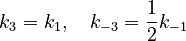
With these assumptions, the three rate constants  and
and  must be estimated. Each of these can be fitted with two adjustable model parameters, assuming an Arrhenius temperature dependence. That is

Here  is the gas constant and
  is the reaction temperature in Kelvins. The parameters
  , given in
 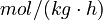 , represent the pre-exponential factors and the
  , with unit
  , are the activation energies.
Mathematical formulation
The chemical processes  can be expressed mathematically as six differential equations and four algebraic equations:
![\begin{align}
\dot{y}_1 &= -k_2 y_8 y_2 && \quad (1),(h) \\
\dot{y}_2 &= -k_1 y_6 y_2 + k_{-1} y_{10} - k_2 y_8 y_2 && \quad (2),(e) \\
\dot{y}_3 &= k_2 y_8 y_2 + k_1 y_6 y_4 - \frac{1}{2} k_{-1} y_9 && \quad (3),(i) \\
\dot{y}_4 &= -k_1 y_6 y_4 + \frac{1}{2} k_{-1} y_9 && \quad (4),(f) \\
\dot{y}_5 &= k_1 y_6 y_2 - k_{-1} y_{10} && \quad (5),(g) \\
\dot{y}_6 &= -k_1 (y_6 y_2 + y_6 y_4) + k_{-1} (y_{10} + \frac{1}{2} y_9) && \quad (6),(d) \\
y_7 &= -\left[ Q^+ \right] + y_6 + y_8 + y_9 + y_{10} && \quad (7),(j)\\
y_8 &= \frac{\theta_8 y_1}{\theta_8 + y_7} && \quad (8),(b)\\
y_9 &= \frac{\theta_9 y_3}{\theta_9 + y_7} && \quad (9),(c)\\
y_{10} &= \frac{\theta_7 y_5}{\theta_7 + y_7} && \quad (10),(a)
\end{align}](https://mintoc.de/images/math/c/d/8/cd8bdeab86edf9fad2f9422431b74bc0.png)
Here the letters in parentheses stand for the corresponding chemical process and the quantity ![\left[Q^+\right]=0.0131](https://mintoc.de/images/math/e/e/f/eefe4f88e9b2b92bf629a01ca55418cf.png) is a constant during the reaction.
The nine parameters form the vector
is a constant during the reaction.
The nine parameters form the vector

The predicted concentrations form the vector

Let  denote the right hand side of equation
  for
for  .
We reformulate the last four algebraic equations as differential ones:
.
We reformulate the last four algebraic equations as differential ones:
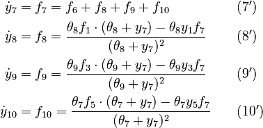
The right hand sides of  and
and  are summarized as the vector-valued function
  .
Moreover, let
.
Moreover, let
Parameters
The initial parameter estimates are:
 |
 |
 |
|
 |
 |
 |
 |
 |
|
 |
|
 |
 |
 |
 |
 |
|
Note that for the calculations all temperatures given in  have to be rescaled to
  by adding
  .
.
There are three datasets for different temperatures , with corresponding starting values
 |
 |
 |
|
|---|---|---|---|
 |
 |
 |
 |
 |
 |
 |
 |
 |
 |
 |
 |
 |
 |
 |
 |
The initial model conditions in addition to those given in the data sets are:
![\begin{array}{l}
y_5 = 0 \\
y_6 = [Q^+] \\
y_7 = \frac{1}{2} \cdot \left( -K_2 + \sqrt{K_2^2 + 4K_2 y_1(0)} \right) \\
y_8 = y_7 \\
y_9 = 0 \\
y_{10} = 0
\end{array}](https://mintoc.de/images/math/9/c/f/9cf55186f9f0f5d6c66de068e18ebd4c.png)
To reduce the intercorrelation between the parameters in the rate constants, we apply the following reparametrization (cf. [4].):

in which 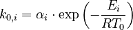 . The reference temperature in
  is chosen as the average over all performed experiments, i.e.,
  . Additionally, we add a logarithmic transformation, which gives rise to the following transformed starting values:
 |
 |
 |
|
 |
 |
|
 |
|
|
|
|
 |
 |
 |
 |
 |
 |
Optimal Experimental Design Problem
To be specified.
We are interested in when to measure (with an upper bound  on the measuring time for each observable).
We define
on the measuring time for each observable).
We define
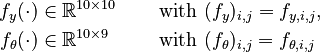
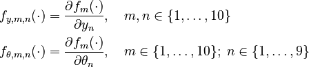
In this approach, we add the so-called sensitivities  . For the differential equations this means

Now we formulate the OED problem as described in [2].
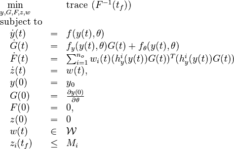
Here 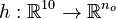 is the observed function. The
evolution of the symmetric matrix
is the observed function. The
evolution of the symmetric matrix ![F: \left[0,t_f \right] \rightarrow \mathbb{R}^{9 \times 9}](https://mintoc.de/images/math/7/1/8/718334578e24248dfbe68e385a44ec30.png) is given by the weighted sum of observability Gramians
is given by the weighted sum of observability Gramians
 for each observed function of states. The weights
  are the (binary) sampling decisions, where
  denotes the decision to perform a measurement at
time
denotes the decision to perform a measurement at
time  .
.
Miscellaneous and Further Reading
To be specified.
References
[1] "Nonlinear Parameter Estimation: a Case Study Comparison" by L. T. Biegler and J. J. Damiano
[2] "Optimal Experimental Design for Universal Differential Equations" by C. Plate, C.J. Martensen and S. Sager
[3] "Parameter estimation in nonlinear systems" by W.J.H. Stortelder
[4] "Parameter Estimation in Nonlinear Dynamical Systems" by Morten Rode Kristensen