Bioreactor

The bioreactor problem describes an substrate that is converted to a product by the biomass in the reactor. It has three states and a control that is describing the feed concentration of the substrate. The problem is taken from the examples folder of the ACADO toolkit described in:

Houska, Boris, Hans Joachim Ferreau, and Moritz Diehl. "ACADO toolkit—An open‐source framework for automatic control and dynamic optimization."
Optimal Control Applications and Methods 32.3 (2011): 298-312.

Originally the problem seems to be motivated by:

VERSYCK, KARINA J., and JAN F. VAN IMPE. "Feed rate optimization for fed-batch bioreactors: From optimal process performance to optimal parameter estimation."
Chemical Engineering Communications 172.1 (1999): 107-124.

Model Formulation

The dynamic model is an ODE model:

$\begin{array}{rcl} \dot{X}&=&-DX+\mu X \\ \dot{S}&=& D(S_{f}-S)-\mu /Y_{xs} X \\ \dot{P}&=&-DP+ (\alpha \mu +\beta) X. \end{array}$

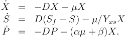
The three states describe the concentration of the biomass ($X$), the substrate ($S$), and the product ($P$) in the reactor. In steady state the feed and outlet are equal and dilute all three concentrations with a ratio $D$. The biomass grows with a rate $\mu$, while it eats up the substrate with the rate $\mu/Y_{xs}$ and produces product at a rate $(\alpha \mu +\beta)$. The rate $\mu$ is given by:

$\mu = \mu_{m}*(1-P/P_{m})*S/(K_m+S+S^2/K_i)$

The fixed parameters (constants) of the model are as follows.

Parameters

Name	Symbol	Value	Unit
Dilution	$D$	0.15	[-]
Rate coefficient	$K_i$	22	[-]
Rate coefficient	$K_m$	1.2	[-]
Rate coefficient	$P_m$	50	[-]
Substrate to Biomass rate	$Y_{xs}$	0.4	[-]
Linear slope	$\alpha$	2.2	[-]
Linear intercept	$\beta$	0.2	[-]
Maximal growth rate	$\mu_m$	0.48	[-]

Optimal Control Problem

Writing shortly for the states in vector notation 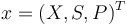$x=(X,S,P)^T$ the OCP reads:

$\begin{array}{cl} \displaystyle \min_{x,S_f} & J(x,S_f)\\[1.5ex] \mbox{s.t.} & \dot{x} = f(x,S_f), \forall \, t \in [0,48]\\ & x(0) = (6.5,12,22)^T \\ & x \in \R^3,\,S_f \in [28.7,40]. \end{array}$

Objective

$J(x,S_f)=\int_0^{48}D(S_f-P)^2dt$

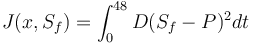
Reference Solution

Here we present the reference solution of the reimplemented example in the ACADO code generation with matlab. The source code is given in the next section.

• Reference solution
• 

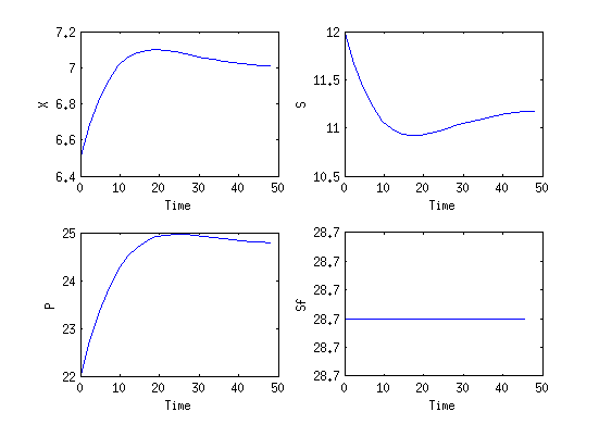
  Optimal solution for the ACADO example.

Source Code

Model descriptions are available in

• ACADO code at Bioreactor (ACADO)

This is the implementation of the ACADO bioreactor example with the matlab interface and the code generation of ACADO.

% implements the bioreactor example of ACADO for the matlab interface and
% the code generation

clc;
clear all;
close all;

Ts = 0.1;
EXPORT = 1;

%% Variables
DifferentialState X S P;
Control Sf;

n_XD = length(diffStates);
n_U = length(controls);

%% Constants
D       = 0.15;
Ki      = 22.0;
Km      = 1.2 ; 
Pm      = 50.0;
Yxs     = 0.4 ;
alpha   = 2.2 ;
beta    = 0.2 ;
mum     = 0.48;
Sfmin   = 28.7;
Sfmax   = 40.0;
t_start =  0.0;
t_end   = 48.0;
N = 20;

%% Differential Equation
mu = mum*(1-P/Pm)*S/(Km+S+S^2/Ki);

f = dot([X;S;P]) == [-D*X+mu*X;...
                      D*(Sf-S)-(mu/Yxs)*X;...
		             -D*P+(alpha*mu+beta)*X];

% output
h = P-Sf;
hN = P;

%% MPCexport
acadoSet('problemname', 'mpc');

ocp = acado.OCP( t_start, t_end, N );

W_mat = D;
WN_mat = D;
W = acado.BMatrix(W_mat);
WN = acado.BMatrix(WN_mat);

ocp.minimizeLSQ( W, h );
ocp.minimizeLSQEndTerm( WN, hN );

ocp.subjectTo( Sfmin <= Sf <= Sfmax );
ocp.setModel(f);

mpc = acado.OCPexport( ocp );
mpc.set( 'HESSIAN_APPROXIMATION',       'GAUSS_NEWTON'      );
mpc.set( 'DISCRETIZATION_TYPE',         'MULTIPLE_SHOOTING' );
mpc.set( 'SPARSE_QP_SOLUTION',          'FULL_CONDENSING_N2');
mpc.set( 'INTEGRATOR_TYPE',             'INT_IRK_GL4'       );
mpc.set( 'NUM_INTEGRATOR_STEPS',        10*N                 );
mpc.set( 'QP_SOLVER',                   'QP_QPOASES'    	);
mpc.set( 'HOTSTART_QP',                 'NO'             	);
mpc.set( 'LEVENBERG_MARQUARDT', 		 1e-10				);

if EXPORT
    mpc.exportCode( 'export_MPC' );
    copyfile('../../../../../../external_packages/qpoases', 'export_MPC/qpoases')
    
    cd export_MPC
    make_acado_solver('../acado_MPCstep')
    cd ..
end

%% CONSTANTS FOR OPTIMIZATION
X0 = [6.5 12.0 22.0];
input.x0=X0';
Xref = [0 0 0];
input.x = repmat(Xref,N+1,1);
Xref = repmat(Xref,N,1);
input.od = [];

Uref = zeros(N,n_U);
input.u = Uref;

input.y = 0*ones(N,1);
input.yN = 0;

input.W = D;
input.WN = D;

%% SOLVER LOOP (SQP - Gauss newton)
display('------------------------------------------------------------------')
display('               SOLVER Loop'                                    )
display('------------------------------------------------------------------')



for i=1:20
    tic
    % Solve NMPC OCP
    output = acado_MPCstep(input);
    
    input.x=output.x;
    input.u=output.u;

    disp([' (RTI step: ' num2str(output.info.cpuTime*1e6) ' µs)'])

end

%% PLOT RESULTS

% States
figure(1)
plot([t_start:t_end/N:t_end],output.x)
ylabel('States')
xlabel('Time')
legend('X','S','P')

% Control
figure(2)
plot([t_start:t_end/N:t_end-t_end/N],output.u)
ylabel('Control (Sf)')
xlabel('Time')

% one figure for all
figure(3)
subplot(2,2,1)
plot([t_start:t_end/N:t_end],output.x(:,1))
ylabel('X')
xlabel('Time')
subplot(2,2,2)
plot([t_start:t_end/N:t_end],output.x(:,2))
ylabel('S')
xlabel('Time')
subplot(2,2,3)
plot([t_start:t_end/N:t_end],output.x(:,3))
ylabel('P')
xlabel('Time')
subplot(2,2,4)
plot([t_start:t_end/N:t_end-t_end/N],output.u)
ylabel('Sf')
xlabel('Time')