Difference between revisions of "Bioreactor"
TobiasWeber (Talk | contribs) |
FelixMueller (Talk | contribs) |
||
| (73 intermediate revisions by 3 users not shown) | |||
| Line 1: | Line 1: | ||
| − | + | {{Dimensions | |
| + | |nd = 1 | ||
| + | |nx = 3 | ||
| + | |nu = 1 | ||
| + | |nc = 2 | ||
| + | |nre = 3 | ||
| + | }} | ||
| − | Houska, Boris, Hans Joachim Ferreau, and Moritz Diehl. "ACADO toolkit—An open‐source framework for automatic control and dynamic optimization." | + | The bioreactor problem describes an substrate that is converted to a product by the biomass in the reactor. It has three states and a control that is describing the feed concentration of the substrate. The problem is taken from the examples folder of the ACADO toolkit described in: |
| + | <bib id="Houska2011a" /> | ||
| + | |||
| + | Houska, Boris, Hans Joachim Ferreau, and Moritz Diehl. | ||
| + | "ACADO toolkit—An open‐source framework for automatic control and dynamic optimization." | ||
Optimal Control Applications and Methods 32.3 (2011): 298-312. | Optimal Control Applications and Methods 32.3 (2011): 298-312. | ||
| − | Originally | + | Originally the problem seems to be motivated by: |
| + | <bib id="Versyck1999" /> | ||
| − | VERSYCK, KARINA J., and JAN F. VAN IMPE. "Feed rate optimization for fed-batch bioreactors: From optimal process performance to optimal parameter estimation." | + | VERSYCK, KARINA J., and JAN F. VAN IMPE. |
| + | "Feed rate optimization for fed-batch bioreactors: From optimal process performance to optimal parameter estimation." | ||
Chemical Engineering Communications 172.1 (1999): 107-124. | Chemical Engineering Communications 172.1 (1999): 107-124. | ||
| Line 18: | Line 30: | ||
\dot{X}&=&-DX+\mu X \\ | \dot{X}&=&-DX+\mu X \\ | ||
\dot{S}&=& D(S_{f}-S)-\mu /Y_{xs} X \\ | \dot{S}&=& D(S_{f}-S)-\mu /Y_{xs} X \\ | ||
| − | \dot{P}&=&-DP+ (\alpha \mu +\beta) X | + | \dot{P}&=&-DP+ (\alpha \mu +\beta) X. |
\end{array} | \end{array} | ||
</math> | </math> | ||
</p> | </p> | ||
| − | The | + | The right-hand side of these equations will be summed up in <math> f(x, S_f) </math>. |
| − | + | The three states describe the concentration of the biomass (<math>X</math>), the substrate (<math>S</math>), and the product (<math>P</math>) in the reactor. In steady state the feed and outlet are equal and dilute all three concentrations with a ratio <math>D</math>. The biomass grows with a rate | |
| + | <math>\mu</math>, while it eats up the substrate with the rate <math>\mu/Y_{xs}</math> and produces product at a rate <math>(\alpha \mu +\beta)</math>. The rate <math>\mu</math> is given by: | ||
| + | <math>\mu = \mu_{m}*(1-P/P_{m})*S/(K_m+S+S^2/K_i)</math> | ||
| − | The | + | The fixed parameters (constants) of the model are as follows. |
{| class="wikitable" | {| class="wikitable" | ||
| − | |+ | + | |+Parameters |
|- | |- | ||
|Name | |Name | ||
| Line 38: | Line 52: | ||
|Unit | |Unit | ||
|- | |- | ||
| − | | | + | |Dilution |
| − | |<math> | + | |<math>D</math> |
| − | | | + | |0.15 |
|[-] | |[-] | ||
| + | |- | ||
| + | |Rate coefficient | ||
| + | |<math>K_i</math> | ||
| + | |22 | ||
| + | |[-] | ||
| + | |- | ||
| + | |Rate coefficient | ||
| + | |<math>K_m</math> | ||
| + | |1.2 | ||
| + | |[-] | ||
| + | |- | ||
| + | |Rate coefficient | ||
| + | |<math>P_m</math> | ||
| + | |50 | ||
| + | |[-] | ||
| + | |- | ||
| + | |Substrate to Biomass rate | ||
| + | |<math>Y_{xs}</math> | ||
| + | |0.4 | ||
| + | |[-] | ||
| + | |- | ||
| + | |Linear slope | ||
| + | |<math>\alpha</math> | ||
| + | |2.2 | ||
| + | |[-] | ||
| + | |- | ||
| + | |Linear intercept | ||
| + | |<math>\beta</math> | ||
| + | |0.2 | ||
| + | |[-] | ||
| + | |- | ||
| + | |Maximal growth rate | ||
| + | |<math>\mu_m</math> | ||
| + | |0.48 | ||
| + | |[-] | ||
| + | |- | ||
|} | |} | ||
| − | + | == Mathematical formulation == | |
| + | |||
| + | Writing shortly for the states in vector notation <math>x=(X,S,P)^T</math> the OCP reads: | ||
| + | |||
| + | <p> | ||
| + | <math> | ||
| + | \begin{array}{clcl} | ||
| + | \displaystyle \min_{x,S_f} & J(x,S_f)\\[1.5ex] | ||
| + | \mbox{s.t.} | ||
| + | & \dot{x} & = & f(x,S_f)\\ | ||
| + | & x(0) & = & (6.5,12,22)^T \\ | ||
| + | & S_f & \in &[28.7,40]. | ||
| + | \end{array} | ||
| + | </math> | ||
| + | </p> | ||
| + | |||
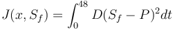
| + | === Objective === | ||
| + | <p> | ||
| + | <math> | ||
| + | J(x,S_f)=\int_0^{48}D(S_f-P)^2dt | ||
| + | </math> | ||
| + | </p> | ||
| + | |||
| + | == Reference Solution == | ||
| + | |||
| + | Here we present the reference solution of the reimplemented example in the ACADO code generation with matlab. The source code is given in the next section. | ||
| + | |||
| + | <gallery caption="Reference solution" widths="551px" heights="390px" perrow="1"> | ||
| + | Image:ACADO_bioreactor.png| Optimal solution for the ACADO example. | ||
| + | </gallery> | ||
| + | |||
| + | == Source Code == | ||
| + | |||
| + | Model descriptions are available in | ||
| + | |||
| + | * [[:Category:ACADO | ACADO code]] at [[Bioreactor (ACADO)]] | ||
| + | |||
| + | <!--List of all categories this page is part of. List characterization of solution behavior, model properties, ore presence of implementation details (e.g., AMPL for AMPL model) here --> | ||
| + | [[Category:MIOCP]] [[Category: ODE model]] [[Category:Chemical engineering]] | ||
| + | [[Category:Bang bang]] | ||
Latest revision as of 10:27, 27 July 2016
| Bioreactor | |
|---|---|
| State dimension: | 1 |
| Differential states: | 3 |
| Continuous control functions: | 1 |
| Path constraints: | 2 |
| Interior point equalities: | 3 |
The bioreactor problem describes an substrate that is converted to a product by the biomass in the reactor. It has three states and a control that is describing the feed concentration of the substrate. The problem is taken from the examples folder of the ACADO toolkit described in: [Houska2011a]The entry doesn't exist yet.
Houska, Boris, Hans Joachim Ferreau, and Moritz Diehl.
"ACADO toolkit—An open‐source framework for automatic control and dynamic optimization."
Optimal Control Applications and Methods 32.3 (2011): 298-312.
Originally the problem seems to be motivated by: [Versyck1999]The entry doesn't exist yet.
VERSYCK, KARINA J., and JAN F. VAN IMPE.
"Feed rate optimization for fed-batch bioreactors: From optimal process performance to optimal parameter estimation."
Chemical Engineering Communications 172.1 (1999): 107-124.
Contents
Model Formulation
The dynamic model is an ODE model:
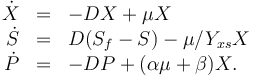
The right-hand side of these equations will be summed up in  .
.
The three states describe the concentration of the biomass ( ), the substrate (
 ), and the product (
 ) in the reactor. In steady state the feed and outlet are equal and dilute all three concentrations with a ratio
  . The biomass grows with a rate
 , while it eats up the substrate with the rate
  and produces product at a rate
  . The rate is given by:

The fixed parameters (constants) of the model are as follows.
| Name | Symbol | Value | Unit |
| Dilution |
|
0.15 | [-] |
| Rate coefficient | 
|
22 | [-] |
| Rate coefficient | 
|
1.2 | [-] |
| Rate coefficient | 
|
50 | [-] |
| Substrate to Biomass rate | 
|
0.4 | [-] |
| Linear slope | 
|
2.2 | [-] |
| Linear intercept | 
|
0.2 | [-] |
| Maximal growth rate | 
|
0.48 | [-] |
Mathematical formulation
Writing shortly for the states in vector notation  the OCP reads:
![\begin{array}{clcl}
\displaystyle \min_{x,S_f} & J(x,S_f)\\[1.5ex]
\mbox{s.t.}
& \dot{x} & = & f(x,S_f)\\
& x(0) & = & (6.5,12,22)^T \\
& S_f & \in &[28.7,40].
\end{array}](https://mintoc.de/images/math/8/8/e/88e448fa43ddbb22c56b967ef453bc16.png)
Objective
Reference Solution
Here we present the reference solution of the reimplemented example in the ACADO code generation with matlab. The source code is given in the next section.
- Reference solution
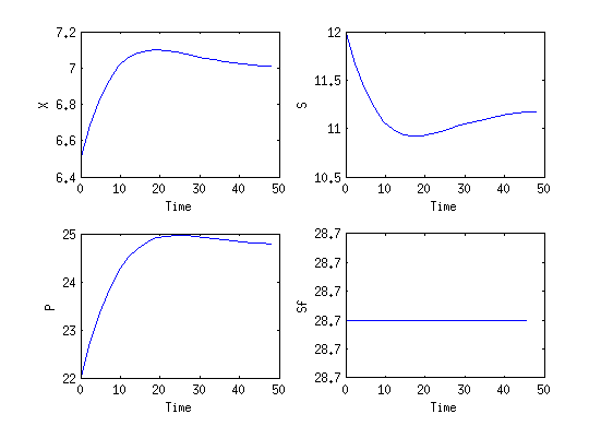
Optimal solution for the ACADO example.

Source Code
Model descriptions are available in