Difference between revisions of "Cushioned Oscillation"
(→Model formulation) |
FelixMueller (Talk | contribs) |
||
| (15 intermediate revisions by 3 users not shown) | |||
| Line 1: | Line 1: | ||
| − | The Cushioned Oscillation is a simplified model of time optimal "stopping" of an oscillating object attached to a spring by applying a control and moving it back into the relaxed position and | + | {{Dimensions |
| + | |nd = 1 | ||
| + | |nx = 2 | ||
| + | |nu = 1 | ||
| + | |nc = 2 | ||
| + | |nre = 4 | ||
| + | }}The Cushioned Oscillation is a simplified model of time optimal "stopping" of an oscillating object attached to a spring by applying a control and moving it back into the relaxed position and zero velocity. | ||
== Model formulation == | == Model formulation == | ||
| Line 12: | Line 18: | ||
where <math>x(t)</math> denotes the deviation to the relaxed position and <math> v(t)=\dot x (t) </math> the velocity of the oscillating object. | where <math>x(t)</math> denotes the deviation to the relaxed position and <math> v(t)=\dot x (t) </math> the velocity of the oscillating object. | ||
| − | |||
| − | |||
Through external force, the object has been put into an initial state : | Through external force, the object has been put into an initial state : | ||
| − | |||
<math>(x(0),v(0)) = (x_0,v_0)</math> | <math>(x(0),v(0)) = (x_0,v_0)</math> | ||
| − | |||
The goal is to reset position and velocity of the object as fast as possible, meaning: | The goal is to reset position and velocity of the object as fast as possible, meaning: | ||
| − | |||
<math>(x(t_f),v(t_f)) = (0,0)</math>, | <math>(x(t_f),v(t_f)) = (0,0)</math>, | ||
| − | |||
| − | |||
with the objective function: | with the objective function: | ||
| − | |||
<math>\min\limits_{t_f} t_f</math> | <math>\min\limits_{t_f} t_f</math> | ||
| − | == Optimal Control Problem | + | == Optimal Control Problem Formulation == |
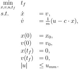
The above results in the following OCP | The above results in the following OCP | ||
| + | <math> \begin{array}{llll} | ||
| − | + | \min\limits_{x,v,u,t_f} & t_f & & \\ | |
| − | + | ||
| − | + | s.t. & \dot x & = v,\\ | |
| − | + | & \dot v & = \frac{1}{m}(u - c \cdot x),\\ | |
\\ | \\ | ||
| − | + | & x(0) & = x_0,\\ | |
| − | & x(0)=x_0,\\ | + | & v(0) & = v_0,\\ |
| − | + | & x(t_f) & = 0,\\ | |
| − | & v(0)=v_0,\\ | + | & v(t_f) & = 0,\\ |
| − | + | & |u| & \le u_{mm}.\\ | |
| − | & x(t_f)=0,\\ | + | |
| − | + | ||
| − | & v(t_f)=0, | + | |
| − | + | ||
| − | \\ | + | |
| − | & | + | |
| − | + | ||
| − | + | ||
\end{array}</math> | \end{array}</math> | ||
| Line 63: | Line 53: | ||
== Parameters and Reference Solution == | == Parameters and Reference Solution == | ||
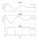
| + | The following parameters were used, to create the reference solution below, with an almost optimal final time <math> t_f = 8.98 s</math>: | ||
| − | + | <math> m=5, </math> | |
| − | + | ||
| − | <math> m= | + | |
| − | + | ||
<math> c=10, </math> | <math> c=10, </math> | ||
| − | |||
<math> x_0=2, </math> | <math> x_0=2, </math> | ||
| − | |||
<math> v_0=5, </math> | <math> v_0=5, </math> | ||
| + | <math> u_{mm}=5.</math> | ||
| − | + | == Reference Solution == | |
| − | + | ||
| − | + | ||
<gallery caption="Reference solution plots" widths="180px" heights="140px" perrow="1"> | <gallery caption="Reference solution plots" widths="180px" heights="140px" perrow="1"> | ||
| − | Image: | + | Image:Ref_sol_plot_cushioned_oscillation_m5.png| States and Controls |
</gallery> | </gallery> | ||
| − | + | The OCP was solved within MATLAB R2015b, using the TOMLAB Optimization Package. PROPT reformulates such problems with the direct collocation approach (n=80 collocation points) and automatically finds a suiting solver included in the TOMLAB Optimization Package (in this case, SNOPT was used). | |
| − | The OCP was solved within MATLAB R2015b, using the TOMLAB Optimization Package. PROPT reformulates such problems with the direct collocation | + | |
| − | + | ||
| − | + | ||
| − | + | ||
== Source Code == | == Source Code == | ||
| − | + | * A MATLAB script using [[:Category:TomDyn/PROPT | PROPT]] can be found in: [[Cushioned Oscillation (PROPT)]] | |
| − | + | ||
| − | [[Category:TomDyn/PROPT]] [[Cushioned Oscillation (PROPT)]] | + | |
== References == | == References == | ||
| − | [[Category:MIOCP]] | + | [[Category:MIOCP]] |
| + | [[Category:Bang bang]] | ||
| + | [[Category:ODE model]] | ||
| + | [[Category: Minimum time]] | ||
Latest revision as of 11:06, 30 June 2016
| Cushioned Oscillation | |
|---|---|
| State dimension: | 1 |
| Differential states: | 2 |
| Continuous control functions: | 1 |
| Path constraints: | 2 |
| Interior point equalities: | 4 |
The Cushioned Oscillation is a simplified model of time optimal "stopping" of an oscillating object attached to a spring by applying a control and moving it back into the relaxed position and zero velocity.
Contents
Model formulation
An object with mass  is attached to a spring with stiffness constant
  .
.
If the resetting spring force is proportional to the deviation  , an oscillation, induced by an external force
  , satisfies:
 (which is equivalent to
  )
)
where  denotes the deviation to the relaxed position and
  the velocity of the oscillating object.
Through external force, the object has been put into an initial state :
The goal is to reset position and velocity of the object as fast as possible, meaning:
 ,
,
with the objective function:

Optimal Control Problem Formulation
The above results in the following OCP
Parameters and Reference Solution
The following parameters were used, to create the reference solution below, with an almost optimal final time  :
:


Reference Solution
- Reference solution plots
States and Controls

The OCP was solved within MATLAB R2015b, using the TOMLAB Optimization Package. PROPT reformulates such problems with the direct collocation approach (n=80 collocation points) and automatically finds a suiting solver included in the TOMLAB Optimization Package (in this case, SNOPT was used).
Source Code
- A MATLAB script using PROPT can be found in: Cushioned Oscillation (PROPT)