Difference between revisions of "LinearMetabolic"

LinearMetabolic
State dimension:	1
Differential states:	4
Discrete control functions:	3
Path constraints:	2
Interior point inequalities:	2
Interior point equalities:	5

Revision as of 08:46, 20 October 2023

The Linear Metabolic problem is a generalized inverse optimal control problem formulated and investigated in [Tsiantis2018]Author: Tsiantis, Nikolaos; Balsa-Canto, Eva; Banga, Julio R
Journal: Bioinformatics
Number: 14
Pages: 2433-2440
Title: Optimality and identification of dynamic models in systems biology: an inverse optimal control framework
Volume: 34
Year: 2018
. It tries to identify an a priori unknown objective function from data.

The problem is a generalization of the one studied by de Hijas-Liste et al. (2014), where it was considered as a standard optimal control problem (OCP). Here, we take the solution reference of the inner problem as the multi-objective OCP described in de Hijas-Liste et al. (2014), selecting a specific point of the resulting Pareto front. This case study is interesting, because it includes path constraints on the states and the inputs.

A 3-step linear metabolic pathway with mass action kinetics is considered. The differential states $x$ are metabolite concentrations, the time-dependent control functions $u$ are enzyme concentrations, and the model parameters $p$ are kinetic parameters in mass action expressions. Candidate objective functionals $\phi$ are the final time and the time-integral of the intermediate metabolite concentrations. The measurement function is a map to the values of the differential states and comprises measurements of metabolite concentrations. The differential equations are assumed to be fully known as standard mass action kinetics. An inequality path constraint is present (but potentially unknown in such settings) on the inner level and critical from a biological point of view: limitations due to molecular crowding impose an upper bound on the maximum total concentration of enzymes (controls) at any given time. Boundary conditions are fixed initial and terminal values of the metabolite concentrations.

Mathematical formulation

Under construction...

The gIOC is given by

   $\displaystyle \min_{(p, w, x^*, u^*, T^*)} \; \| x^* - \eta \|$ 
     subject to
      $(x^*,u^*, T^*) \in \displaystyle \arg \min_{x, u, T} w_1 \cdot \int_{0}^{T} (x_2 + x_3) \, dt + w_2 \cdot \int_{0}^{T} 1 \,dt$ 
                subject to
                 $\begin{array}{rcl} \dot{x_1}(t) &=& \displaystyle 0 \\ \dot{x_2}(t) &=& \displaystyle p_1 \cdot x_1 \cdot u_1 - p_2 \cdot x_2 \cdot u_2 \\ \dot{x_3}(t) &=& \displaystyle p_2 \cdot x_2 \cdot u_2 - p_3 \cdot x_3 \cdot u_3 \\ \dot{x_4}(t) &=& \displaystyle p_3 \cdot x_3 \cdot u_3 \\ x(0) &=& (1, 0, 0, 0) \\ x_4(T) &=& 0.9 \\ x_i(t) &\ge& 0 \; \forall \; i \in \{1,2,3,4\} \\ u_i(t) &\in& [0,1] \; \forall \; i \in \{1,2,3\} \\ w_1, w_2 \in [0,1] \\ w_1 + w_2 = 1 \end{array}$

Here the four differential states and three control functions stand for the metabolite concentrations ( $x_1, x_2, x_3, x_4$ ) and the enzyme concentrations ( $u_1, u_2, u_3$ ). The objective function candidates are the sum of intermediate metabolite concentrations and the transition time. The parameters ( $k_1, k_2, k_3$ ) are kinetic parameters in mass action expressions.

Data

Data
weights	parameters	noise	data
[0.232, 0.768]	[1,1,1]	0	[[1.0, 1.0, 1.0, 1.0, 1.0, 1.0, 1.0, 1.0, 1.0, 1.0, 1.0, 1.0, 1.0, 1.0, 1.0, 1.0, 1.0, 1.0, 1.0, 1.0, 1.0], [0, 0.215, 0.4298, 0.6446, 0.8593, 1.074, 1.2885, 1.503, 1.6591, 1.3381, 1.0792, 0.8704, 0.7021, 0.5662, 0.4849, 0.4846, 0.4844, 0.4842, 0.484, 0.4838, 0.4836], [0, 0.0, 0.0002, 0.0004, 0.0007, 0.001, 0.0015, 0.002, 0.0391, 0.36, 0.6186, 0.827, 0.9948, 1.1301, 1.1405, 0.92, 0.7423, 0.5989, 0.4832, 0.3899, 0.3147], [0, 0.0, 0.0, 0.0, 0.0, 0.0, 0.0, 0.0, 0.0, 0.0001, 0.0004, 0.0008, 0.0013, 0.0019, 0.0729, 0.2935, 0.4715, 0.6152, 0.731, 0.8245, 0.9]]
[0.232, 0.768]	[1,1,1]	0.2	[[1. ,0.9590812 ,0.82266497,0.95877308,0.60614596,1.20781224, 0.92205471,1.0215116 ,0.89080449,1.05747735,1.04019676,1.06665347, 0.78545416,1.17084962,1.08658091,1.01467309,0.91098074,1.10349004, 0.83411596,0.73187308,0.70399766],[0. ,0.37493181,0.10514573,0.79448823,0.44666767,1.19676033, 1.14532119,1.64453389,1.93572019,1.37435635,0.92790967,1.11928728, 0.52061388,0.43837628,0.31518386,0.50300858,0.52891948,0.74255261, 0.07589526,0.64051491,0.47184952],[ 0. , 0.23680072, 0.05047157,-0.03770305, 0.34603556,-0.45259701, 0.25340369, 0.25177705, 0.16210031, 0.34367395, 0.96197961, 1.10224845, 1.21656021, 1.38442255, 1.02149302, 0.68818982, 0.7921558 , 0.32238544, 0.30229594, 0.43876605, 0.22073986],[ 0. ,-0.01591557,-0.12432336,-0.17669569,-0.21325853,-0.2489822 , -0.22989873,-0.0564741 ,-0.19961696,-0.16036058,-0.04386598, 0.25004781, -0.07279584, 0.09573081,-0.12329308,-0.03451486, 0.0173815 , 0.79895333, 0.8178261 , 0.53498205, 1.1021996 ]]
[0,1]	[1,1,1]	0	[[1, 1, 1, 1, 1, 1, 1, 1, 1, 1, 1, 1, 1, 1, 1, 1, 1, 1, 1, 1, 1], [0, 0.211317, 0.422635, 0.633952, 0.845269, 1.05659, 1.2679, 1.47922, 1.69054, 1.90186, 1.95601, 1.58342, 1.2818, 1.03764, 0.839981, 0.685458, 0.685458, 0.685458, 0.685458, 0.685458, 0.685458], [0, 3.40252e-10, 2.02262e-09, 6.04129e-09, 1.32631e-08, 2.47434e-08, 4.23248e-08, 6.98021e-08, 1.16723e-07, 2.20847e-07, 0.103509, 0.476095, 0.777716, 1.02188, 1.21954, 1.36367, 1.10391, 0.893635, 0.72341, 0.58561, 0.474061], [0, 2.79389e-19, 2.05361e-18, 7.26553e-18, 1.82666e-17, 3.77412e-17, 6.87107e-17, 1.14894e-16, 1.82155e-16, 2.86358e-16, 3.73778e-11, 7.31532e-10, 5.75723e-09, 2.28945e-08, 7.3467e-08, 0.0103927, 0.270148, 0.480425, 0.65065, 0.78845, 0.9]]
[0,1]	[1,1,1]	0.1	[[1. ,0.98392517,1.02825092,1.0127091 ,1.21814838,1.03987996, 1.17367563,1.0721497 ,1.11254303,0.91560159,0.92664064,0.93069442, 1.01285111,1.10017347,0.9952073 ,1.05616016,1.12564585,1.02743444, 0.93306189,1.04808763,0.87659083],[0. ,0.19112834,0.6016258 ,0.70894548,0.86077117,0.95316772, 1.12244906,1.51535841,1.48548905,1.87282215,2.13181979,1.48523121, 1.14624017,1.06839771,0.8838448 ,0.72466348,0.61379013,0.70096009, 0.73549769,0.62452413,0.61907767],[ 0. , 0.04514029,-0.06510522,-0.00304812,-0.01620013, 0.006101 , 0.04992798, 0.29317191, 0.11305888, 0.2285637 , 0.26142926, 0.50457228, 0.87829835, 0.90900075, 1.32279588, 1.42225272, 1.18086941, 0.67720058, 0.61562944, 0.6339817 , 0.36613472],[ 0. ,-0.13882966, 0.18200648,-0.06629627,-0.01496019, 0.21349797, -0.10124824,-0.05505019, 0.23235014, 0.09448396, 0.06059911,-0.12137716, -0.00781841, 0.04355511, 0.1369212 ,-0.13011339, 0.2027646 , 0.51512985, 0.65331917, 0.78324169, 0.81304223]]

Examples

Here are two plots with noise free data for weights [0.232, 0.768] to compare with the solution of different optimal control problems.

Solution plots
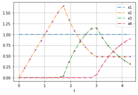
OCP with weights [0.232, 0.768].
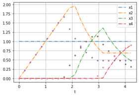
OCP with weights [0,1].

References

[Tsiantis2018]

Tsiantis, Nikolaos; Balsa-Canto, Eva; Banga, Julio R (2018): Optimality and identification of dynamic models in systems biology: an inverse optimal control framework. Bioinformatics, 34, 2433-2440

@@ Line 21: / Line 21: @@
 The gIOC is given by
-<p>
+   <math>
-<math>
     \displaystyle \min_{(p, w, x^*, u^*, T^*)} \; \| x^* - \eta \|
     </math>
@@ Line 44: / Line 43: @@
                   \end{array}
                   </math>
-</p>
 Here the four differential states and three control functions stand for the metabolite concentrations (<math> x_1, x_2, x_3, x_4 </math>) and the enzyme concentrations (<math> u_1, u_2, u_3 </math>). The objective function candidates are the sum of intermediate metabolite concentrations and the transition time. The parameters (<math> k_1, k_2, k_3 </math>) are kinetic parameters in mass action expressions.
@@ Line 118: / Line 117: @@
 </gallery>
-== Parameters ==
-These fixed values are used within the model.
-{| class="wikitable"
-|+Parameters
-|-
-|Name
-|Symbol
-|Value
-|Unit
-|-
-|Coefficient of reduction
-|<math>K_r</math>
-|10
-|[-]
-|-
-|Air density
-|<math>\rho</math>
-|1.293
-|<math> kg/m^3 </math>
-|-
-|Aerodynamic coefficient
-|<math>C_x</math>
-|0.4
-|[-]
-|-
-|Area in the front of the vehicle
-|<math>S</math>
-|2
-|<math> m^2  </math>
-|-
-|Radius of the wheel
-|<math>r</math>
-|0.33
-|<math> m </math>
-|-
-|Constant representing the friction of the wheels on the road
-|<math>K_f </math>
-|0.03
-|[-]
-|-
-|Coefficient of the motor torque
-|<math>K_m</math>
-|0.27
-|[-]
-|-
-|Inductor resistance
-|<math>R_m</math>
-|0.03
-|<math> Ohms </math>
-|-
-|inductance of the rotor
-|<math>L_m</math>
-|0.05
-|[-]
-|-
-|Mass
-|<math>M</math>
-|250
-|<math> kg </math>
-|-
-|Gravity constant
-|<math>g</math>
-|9,81
-|[-]
-|-
-|Battery voltage
-|<math>V_{alim}</math>
-|150
-|<math> V </math>
-|-
-|Resistance of the battery
-|<math>R_{bat}</math>
-|0.05
-|<math> Ohms </math>
-|-
-|}
-== Reference Solutions ==
-We look at the particular instance of our problem with <math> t_f = 10s </math>and target set <math> \mathcal{T} = \mathbb{R} \times \mathbb{R}  \times \{100\} \times \mathbb{R} </math>, in which the car needs to cover 100m in 10s.
-Figure 1 shows a plot of the differential states of the optimal trajectory of the relaxed problem (i.e. <math> u \in [-1,1] </math>instead of <math> u \in \{-1,1\} </math>) for <math> N = 1000, N </math>being the number of time discretization points. The current <math>  x_0 </math>increases to its maximal value of 150A, stays there for a certain time, decreases on its minimal value of -150A, stays on this value and eventually increases slightly. This behavior corresponds to the different arcs bang, path-constrained, singular, path-constrained, bang and can be observed also in Figure 2. It shows the corresponding switching function and the optimal control. Note that the plots show data from the solution with the indirect approach.
-Applying the sum up rounding strategy results in an integer-feasible chattering solution.
-The resulting primal states are shown in Figure 3. One observes the high-frequency zig-zagging of the current  <math> x_0 </math>that results from the fast switches in the control.
-The direct and indirect approaches are local optimization techniques and only provide upper bounds for the relaxed problem and hence for the original problem. Here the indirect solution of the relaxed problem gives us a bound of <math> x_3(t_f) = 22777.2 </math>.
-<gallery caption="Reference solution plots" widths="180px" heights="140px" perrow="3">
- Image:ElectricCar PrimalStates Plot.PNG| Primal states of an optimal trajectory for the relaxed problem on a control discretization grid with <math> N = 1,000 </math>.
- Image:ElectricCar Control PathConstraints SwitchingFunction Plot.PNG| The optimal control and switching function. The dotted vertical lines show the switching times <math> \tau_i </math> where transitions between different kinds of arcs occur.
- Image:ElectricCar PrimalStates SumUpRounding.PNG| Primal states with Sum up rounding on grid with <math> \Delta t = 10^{-2} </math>.
-</gallery>
-== Source Code ==
-Model descriptions are available in
-* [[:Category:AMPL | AMPL code]] at [[Electric car problem (AMPL)]]
-== Variants ==
-There are several alternative formulations and variants of the above problem, in particular
-* fixed final velocity, <math> \mathcal{T} = \mathbb{R} \times \{ 50 \frac{K_r}{3.6r} \} \times \{100\} \times \mathbb{R}, t_f = 10s </math>
-* bounded velocity, <math> \mathcal{T} = \mathbb{R} \times \mathbb{R} \times \{100\} \times \mathbb{R}, t_f = 10s, x_2(t) \leq 45 \frac{K_r}{3.6r} \forall t </math>
-* fixed final velocity, bounded velocity, longer time horizon, <math> x_2(t) \leq 30 \frac{K_r}{3.6r} \forall t, \mathcal{T} = \mathbb{R} \times \{ 30 \frac{K_r}{3.6r} \} \times \{100\} \times \mathbb{R}, t_f = 15s </math>.
 == References ==

Difference between revisions of "LinearMetabolic"

Revision as of 08:46, 20 October 2023

Contents

Mathematical formulation

Data

Examples

References

Navigation menu

Personal tools

Namespaces

Variants

Views

More

Search

Navigation

Support

Tools