Difference between revisions of "Oil Shale Pyrolysis"
From mintOC
FelixMueller (Talk | contribs) |
|||
| Line 8: | Line 8: | ||
}} | }} | ||
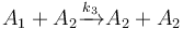
| − | The following problem is an example from the global optimal control literature and was introduced in <bib id="Wen1977" />. | + | The following problem is an example from the global optimal control literature and was introduced in <bib id="Wen1977" />. The process starts with kerogen and is decomposed into pyrolytic bitumen, oil and gas, and residual carbon. The objective is to maximize the fraction of pyrolytic bitumen. There are 5 reactions including: |
| + | <math>A_1 \xrightarrow{k_1} A_2</math> | ||
| + | |||
| + | <math>A_2 \xrightarrow{k_2} A_3</math> | ||
| + | |||
| + | <math>A_1 + A_2 \xrightarrow{k_3} A_2 + A_2</math> | ||
| + | |||
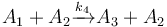
| + | <math>A_1 + A_2 \xrightarrow{k_4} A_3 + A_2</math> | ||
| + | |||
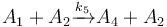
| + | <math>A_1 + A_2 \xrightarrow{k_5} A_4 + A_2</math> | ||
| + | |||
| + | Each reaction is governed by a rate described by: | ||
| + | |||
| + | <math>k_i = k_{i0} \exp{-E_i/RT}, (i=1,2,3,4,5)</math> | ||
== Mathematical formulation == | == Mathematical formulation == | ||
| Line 15: | Line 28: | ||
<math> | <math> | ||
\begin{array}{lll} | \begin{array}{lll} | ||
| − | \displaystyle \min_{ | + | \displaystyle \min_{T} & \displaystyle &-x_1(t_N) \\[1.5ex] |
| − | \mbox{s.t.} & \displaystyle \dot{x} | + | \mbox{s.t.} & \displaystyle \dot{x}_1 &= -k_1x_1-(k_3+k_4+k_5)x_1x_2\\ |
| − | & \displaystyle \dot{x} | + | & \displaystyle \dot{x}_2 &= k_1x_1-k_2x_2 + k_3x_1x_2\\ |
| − | & \displaystyle k_i &= a_i e^{- | + | & \displaystyle \dot{x}_3 &= k_2x_2 + k_4x_1x_2\\ |
| + | & \displaystyle \dot{x}_4 &= k_5x_1x_2\\ | ||
| + | & \displaystyle k_i &= a_i e^{-\frac{b_i}{RT}},\quad \forall i\in \{1,\dots,5\} \\ [1.5ex] | ||
& \displaystyle t &\in \left[t_0,t_N\right] \\ | & \displaystyle t &\in \left[t_0,t_N\right] \\ | ||
| − | & \displaystyle | + | & \displaystyle T(t) &\in \left[698.15K,748.15K\right]\\ |
| − | & \displaystyle x(t_0) &= (1,0)^T\\ | + | & \displaystyle x(t_0) &= (1,0,0,0)^T\\ |
\end{array} | \end{array} | ||
</math> | </math> | ||
| − | |||
| − | |||
| − | |||
| − | |||
| − | |||
| − | |||
== Parameters == | == Parameters == | ||
| − | |||
| − | |||
{| class="wikitable" | {| class="wikitable" | ||
| Line 41: | Line 48: | ||
|Initial value (<math>t_0</math>) | |Initial value (<math>t_0</math>) | ||
|- | |- | ||
| − | |<math> | + | |<math>x_1(t_0)</math> |
|<math>1</math> | |<math>1</math> | ||
|- | |- | ||
| − | |<math> | + | |<math>x_2(t_0)</math> |
| + | |<math>0 </math> | ||
| + | |- | ||
| + | |<math>x_3(t_0)</math> | ||
| + | |<math>0 </math> | ||
| + | |- | ||
| + | |<math>x_4(t_0)</math> | ||
|<math>0 </math> | |<math>0 </math> | ||
|} | |} | ||
| Line 55: | Line 68: | ||
|- | |- | ||
|<math>a_1</math> | |<math>a_1</math> | ||
| − | |<math> | + | |<math>20.3</math> |
|- | |- | ||
|<math>a_2</math> | |<math>a_2</math> | ||
| − | |<math> | + | |<math>37.4</math> |
|- | |- | ||
|<math>a_3</math> | |<math>a_3</math> | ||
| − | |<math> | + | |<math>33.8</math> |
|- | |- | ||
|<math>a_4</math> | |<math>a_4</math> | ||
| − | |<math> | + | |<math>28.2</math> |
|- | |- | ||
|<math>a_5</math> | |<math>a_5</math> | ||
| − | |<math> | + | |<math>31.0</math> |
|- | |- | ||
|<math>b_1</math> | |<math>b_1</math> | ||
| − | |<math> | + | |<math>\exp{8.86}</math> |
|- | |- | ||
|<math>b_2</math> | |<math>b_2</math> | ||
| − | |<math> | + | |<math>\exp{24.25}</math> |
|- | |- | ||
|<math>b_3</math> | |<math>b_3</math> | ||
| − | |<math> | + | |<math>\exp{23.67}</math> |
|- | |- | ||
|<math>b_4</math> | |<math>b_4</math> | ||
| − | |<math> | + | |<math>\exp{18.75}</math> |
|- | |- | ||
|<math>b_5</math> | |<math>b_5</math> | ||
| − | |<math> | + | |<math>\exp{20.7}</math> |
|} | |} | ||
| Line 91: | Line 104: | ||
|Interval | |Interval | ||
|- | |- | ||
| − | |<math> | + | |<math>T(t)</math> |
| − | |[698 | + | |[698.15,748.15] |
|} | |} | ||
| − | |||
| − | |||
== Reference solution == | == Reference solution == | ||
Revision as of 03:49, 15 March 2019
| Oil Shale Pyrolysis | |
|---|---|
| State dimension: | 1 |
| Differential states: | 2 |
| Continuous control functions: | 1 |
| Discrete control functions: | 0 |
| Path constraints: | 4 |
| Interior point equalities: | 2 |
The following problem is an example from the global optimal control literature and was introduced in [Wen1977]The entry doesn't exist yet.. The process starts with kerogen and is decomposed into pyrolytic bitumen, oil and gas, and residual carbon. The objective is to maximize the fraction of pyrolytic bitumen. There are 5 reactions including:


Each reaction is governed by a rate described by:

Mathematical formulation
![\begin{array}{lll}
\displaystyle \min_{T} & \displaystyle &-x_1(t_N) \\[1.5ex]
\mbox{s.t.} & \displaystyle \dot{x}_1 &= -k_1x_1-(k_3+k_4+k_5)x_1x_2\\
& \displaystyle \dot{x}_2 &= k_1x_1-k_2x_2 + k_3x_1x_2\\
& \displaystyle \dot{x}_3 &= k_2x_2 + k_4x_1x_2\\
& \displaystyle \dot{x}_4 &= k_5x_1x_2\\
& \displaystyle k_i &= a_i e^{-\frac{b_i}{RT}},\quad \forall i\in \{1,\dots,5\} \\ [1.5ex]
& \displaystyle t &\in \left[t_0,t_N\right] \\
& \displaystyle T(t) &\in \left[698.15K,748.15K\right]\\
& \displaystyle x(t_0) &= (1,0,0,0)^T\\
\end{array}](https://mintoc.de/images/math/9/6/8/96843c5154d9757d070e55ffc4cf4e7c.png)
Parameters
| Symbol | Initial value ( ) )
|

|

|

|

|

|
|

|
|
| Symbol | Value |

|

|

|

|

|

|

|

|

|

|

|

|

|

|

|

|

|

|

|

|
| Symbol | Interval |

|
[698.15,748.15] |
Reference solution
Coming soon.
Source Code
Model descriptions are not yet available.
References
| [Wen1977] | The entry doesn't exist yet. |