Difference between revisions of "Van der Pol Oscillator (Jump)"
FelixMueller (Talk | contribs) |
FelixMueller (Talk | contribs) |
||
| (8 intermediate revisions by the same user not shown) | |||
| Line 1: | Line 1: | ||
| − | This is an implementation of a slightly modified form of the Van der Pol | + | This is an implementation of a slightly modified form of the [[Van der Pol Oscillator]] problem using [[:category: Julia/JuMP | JuMP]]. |
The problem in question can be stated as follows: | The problem in question can be stated as follows: | ||
| Line 7: | Line 7: | ||
\begin{array}{llclr} | \begin{array}{llclr} | ||
\displaystyle \max_{x, u} & x_3(t_f) \\[1.5ex] | \displaystyle \max_{x, u} & x_3(t_f) \\[1.5ex] | ||
| − | \mbox{s.t.} & \dot{x}_1 | + | \mbox{s.t.} & \dot{x}_1 & = & (1 - x_2^2) x_1 - x_2 + u, \\ |
| − | & \dot{x}_2 | + | & \dot{x}_2 & = & x_1, \\ |
| − | & \dot{x}_3 | + | & \dot{x}_3 & = & x_1^2 + x_2^2 + u^2, \\[1.5ex] |
& x(0) &=& (0, 1, 0)^T, \\ | & x(0) &=& (0, 1, 0)^T, \\ | ||
| − | & u(t) &\in& [-0.3, 1 | + | & u(t) &\in& [-0.3, 1]. |
\end{array} | \end{array} | ||
</math> | </math> | ||
| Line 21: | Line 21: | ||
Although not necessary in JuMP the code was divided into three parts (following AMPL) - model file, data file and run file. The run file calls the other files and performs additional tasks such as printing results. | Although not necessary in JuMP the code was divided into three parts (following AMPL) - model file, data file and run file. The run file calls the other files and performs additional tasks such as printing results. | ||
| − | A reference solution including plots done with JuMP | + | A reference solution including plots done with JuMP can be found below the code! |
| Line 113: | Line 113: | ||
println("Optimal objective value is: ", getObjectiveValue(m)) | println("Optimal objective value is: ", getObjectiveValue(m)) | ||
println("Optimal Solution is: \n", getValue(x), getValue(u))</source> | println("Optimal Solution is: \n", getValue(x), getValue(u))</source> | ||
| + | |||
| + | == Reference solutions == | ||
| + | This solution was computed using JuMP with a collocation method and 300 discretization points (using the code above). The differential equations were solved using the explicit Euler Method. The optimal objective value is 2.902143. | ||
| + | |||
| + | <gallery caption="Reference solution plots" widths="180px" heights="140px" perrow="2"> | ||
| + | File:Vdposc states plot.PNG| Optimal states x1(t), x2(t) and x3(t). | ||
| + | File:Vdposc control plot.PNG| Optimal control u(t). | ||
| + | </gallery> | ||
[[Category: Julia/JuMP]] | [[Category: Julia/JuMP]] | ||
Latest revision as of 13:35, 23 February 2016
This is an implementation of a slightly modified form of the Van der Pol Oscillator problem using JuMP.
The problem in question can be stated as follows:
![\begin{array}{llclr}
\displaystyle \max_{x, u} & x_3(t_f) \\[1.5ex]
\mbox{s.t.} & \dot{x}_1 & = & (1 - x_2^2) x_1 - x_2 + u, \\
& \dot{x}_2 & = & x_1, \\
& \dot{x}_3 & = & x_1^2 + x_2^2 + u^2, \\[1.5ex]
& x(0) &=& (0, 1, 0)^T, \\
& u(t) &\in& [-0.3, 1].
\end{array}](https://mintoc.de/images/math/f/0/6/f06570f2bb0157845839eca4c59785ac.png)
where ![[t_0, t_f] = [0,5]](https://mintoc.de/images/math/3/d/a/3da50823830060b643c0d60aed66e999.png) .
.
The problem was discretized and the ODEs are solved using the explicit Euler method.
Although not necessary in JuMP the code was divided into three parts (following AMPL) - model file, data file and run file. The run file calls the other files and performs additional tasks such as printing results.
A reference solution including plots done with JuMP can be found below the code!
Model file ("vdposc_mod.jl"):
#JuMP implementation of Van der Pol oscillator using collocation
#mod file

#declaring the model
m = Model(solver=IpoptSolver())

#defining variables
@defVar(m, x[ii=1:n_x, tt=1:N])
@defVar(m, L_control <= u[jj = 1:n_u, tt=1:N] <= U_control)

#set objective function
@setObjective(m, Min, x[3,N])

#setting constraints
#starting values
@addConstraint(m, starting_value[ii=1:n_x], x[ii,1] == x_start[ii])

#ODE - solved with explicit euler method (i.e. x_k+1 = x_k + stepsize * f(x_k, t_k))
@addNLConstraint(m, ODE_nonlin[ii=1:1, tt=1:N-1],  x[ii,tt+1] - x[ii,tt] - step_size * ((1 - x[2,tt]^2) * x[1,tt]
 - x[2,tt] + u[1,tt]) == 0)
@addConstraint(m, ODE[ii=2:n_x, tt=1:N-1],  x[ii,tt+1] - x[ii,tt] - step_size * ode_rhs(time_disc[tt], x[:,tt], u[:,tt])[ii]  >= 0)
@addConstraint(m, ODE[ii=2:n_x, tt=1:N-1],  x[ii,tt+1] - x[ii,tt] - step_size * ode_rhs(time_disc[tt], x[:,tt], u[:,tt])[ii]  <= 0)
Data file ("vdposc_dat.jl"):
#JuMP implementation of Van der Pol oscillator using collocation
#dat file

#number of states
n_x = 3;

#number of controls
n_u = 1;

##discretization
#number of shooting intervals / discretization points
N = 300;
#starting / end time
t_start = 0;
t_end = 5;
#time discretization
time_disc = linspace(t_start,t_end, N+1);
step_size = (t_end - t_start)/N;

#starting value
x_start = [0, 1, 0];

#bounds for control
L_control = -0.3;
U_control = 1;


##right hand side of ODE
function ode_rhs(time, state, control)
#give in form f1, f2, f3,...
0,
state[1],
state[1]^2 + state[2]^2 + control[1]^2
end
Run file ("vdposc_run.jl"):
#JuMP implementation of Van der Pol oscillator using collocation
#run file

using JuMP;
using Ipopt;


println("----------------------------------------------------")
println("Time used for data")
@time include("vdposc_dat.jl")
println("----------------------------------------------------")
println("Time used for modeling")
@time include("vdposc_mod.jl")
println("----------------------------------------------------")
println("Time used for solving")
@time solve(m);

println("----------------------------------------------------")
println("----------------------------------------------------")


println("Optimal objective value is: ", getObjectiveValue(m))
println("Optimal Solution is: \n", getValue(x), getValue(u))
Reference solutions
This solution was computed using JuMP with a collocation method and 300 discretization points (using the code above). The differential equations were solved using the explicit Euler Method. The optimal objective value is 2.902143.
- Reference solution plots
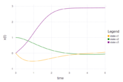
Optimal states x1(t), x2(t) and x3(t).
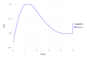
Optimal control u(t).

