Difference between revisions of "Gravity Turn Maneuver"

Gravity Turn Maneuver
State dimension:	1
Differential states:	5
Continuous control functions:	1
Path constraints:	11
Interior point inequalities:	2
Interior point equalities:	7

Latest revision as of 09:29, 27 July 2016

The gravity turn or zero lift turn is a common maneuver used to launch spacecraft into orbit from bodies that have non-negligible atmospheres. The goal of the maneuver is to minimize atmospheric drag by always orienting the vehicle along the velocity vector. In this maneuver, the vehicle's pitch is determined solely by the change of the velocity vector through gravitational acceleration and thrust. The goal is to find a launch configuration and thrust control strategy that achieves a specific orbit with minimal fuel consumption.

Physical description and model derivation

For the purposes of this model, we start with the following ODE system proposed by Culler et. al. in [Culler1957]The entry doesn't exist yet.:

\begin{array}{rcl} \dot{v} &=& \frac{F}{m} - g \cdot \cos \beta \\ v \dot{\beta} &=& g \cdot \sin{\beta} \end{array}

where $v$ is the speed of the vehicle, $g$ is the gravitational acceleration at the vehicle's current altitude, $F$ is the accelerating force and $\beta$ is the angle between the vertical and the vehicle's velocity vector. In the original version of the model, the authors neglect aspects of the problem:

Variation of $g$ over altitude
Decrease of vehicle mass due to fuel consumption
Curvature of the surface
Atmospheric drag

Changes in gravitational acceleration

To account for changes in $g$ , we make the following substitution:

g = g_0 \cdot \left(\frac{r_0}{r_0 + h}\right)^2

where

g_0

is the gravitational acceleration at altitude zero and

r_0

is the distance of altitude zero from the center of the reference body.

Decrease in vehicle mass

To account for changes in vehicle mass, we consider $m$ a differential state with the following derivative:

\dot{m} = -\frac{F}{I_{sp} \cdot g_0}

where

I_{sp}

is the specific impulse of the vehicle's engine. Specific impulse is a measure of engine efficiency. For rocket engines, it directly correlates with the engine's exhaust velocity and may vary with atmospheric pressure, velocity, engine temperature and combustion dynamics. For the purposes of this model, we will assume it to be constant.

The vehicle's fuel reserve is modelled by two parameters: $m_0$ denotes the launch mass (with fuel) and $m_1$ denotes the dry mass (without fuel).

Curvature of the reference body's surface

To accomodate the reference body's curvature, we introduce an additional differential state $\theta$ which represents the change in the vehicle's polar angle with respect to the launch site. The derivative is given by

\dot{\theta} = \frac{v \cdot \sin \beta}{r_0 + h}.

Note that the vertical changes as the vehicle moves around the reference body meaning that the derivative of $\beta$ must be changed as well:

\dot{\beta} = \frac{g \cdot \sin{\beta}}{v} - \frac{v \cdot \sin \beta}{r_0 + h}.

Atmospheric drag

To model atmospheric drag, we assume that the vehicles draf coefficient $c_d$ is constant. The drag force is given by

F_{drag} = \frac{1}{2} \rho A c_d v^2

where $\rho$ is the density of the atmosphere and $A$ is the vehicle's reference area. We assume that atmospheric density decays exponentially with altitude:

\rho = \rho_0 \cdot e^{-\frac{h}{H}}

where $\rho_0$ is the atmospheric density at altitude zero and $H$ is the scale height of the atmosphere. The [drag force] is introduced into the acceleration term:

\dot{v} = \frac{F - F_{drag}}{m} - g \cdot \cos \beta.

Note that if the vehicle is axially symmetric and oriented in such a way that its symmetry axis is parallel to the velocity vector, it does not experience any lift forces. This model is simplified. It does not account for changes in temperature and atmospheric composition with altitude. Also, $c_d$ varies with fluid viscosity and vehicle velocity. Specifically, drastic changes in $c_d$ occur as the vehicle breaks the sound barrier. This is not accounted for in this model.

Mathematical formulation

The resulting optimal control problem is given by

\begin{array}{llcll} \displaystyle \min_{T, m, v, \beta, h, \theta, u} & m_0 - m(T) \\[1.5ex] \mbox{s.t.} & \dot{m} & = & -\frac{F_{max}}{I_{sp} \cdot g_0} \cdot u ,\\ & \dot{v} & = & (F - \frac{1}{2} \rho_0 \cdot e^{-\frac{h}{H}} A c_d v^2) \cdot \frac{1}{m} - g_0 \cdot \left(\frac{r_0}{r_0 + h}\right)^2 \cos \beta ,\\ & \dot{\beta} & = & g_0 \cdot \left(\frac{r_0}{r_0 + h}\right)^2 \cdot \frac{\sin{\beta}}{v} - \frac{v \cdot \sin \beta}{r_0 + h} ,\\ & \dot{h} & = & v \cdot \cos \beta ,\\ & \dot{\theta} & = & \frac{v \cdot \sin \beta}{r_0 + h},\\[1.5ex] & m(0) &=& m_0 , \\ & v(0) &=& \varepsilon , \\ & \beta(0) &\in& \left[ 0,\frac{\pi}{2} \right], \\ & h(0) &=& 0, \\ & \theta(0) &=& 0, \\[1.5ex] & \beta(T) &=& \hat{\beta} , \\ & h(T) &=& \hat{h} , \\ & v(T) &=& \hat{v} , \\[1.5ex] & m(t) &\in& [m_1, m_0] \qquad & \forall t \in [0,T] , \\ & v(t) &\geq& \varepsilon \qquad & \forall t \in [0,T] , \\ & \beta(t) &\in& [0, \pi] \qquad & \forall t \in [0,T] , \\ & h(t) &\geq& 0 \qquad & \forall t \in [0,T] , \\ & \theta(t) &\geq& 0 \qquad & \forall t \in [0,T] , \\[1.5ex] & u(t) &\in& [0,1] \qquad & \forall t \in [0,T] , \\ & T &\in& [T_{min}, T_{max}]. \end{array}

where $F_{max}$ is the maximum thrust of the vehicle's engine and $\varepsilon$ is a small number that is strictly greater than zero. The differential states of the problem are $m, v, \beta, h, \theta$ while $u$ is the control function

Parameters

For testing purposes, the following parameters were chosen:

\begin{array}{rcl} m_0 &=& 11.3 \; t \\ m_1 &=& 1.3 \; t \\ I_{sp} &=& 300 \; s \\ F_{max} &=& 0.6 \; MN \\ c_d &=& 0.021 \\ A &=& 1 \; m^2 \\[1.5ex] g_0 &=& 9.81 \cdot 10^{-3} \, \frac{km}{s^2} \\ r_0 &=& 600.0 \; km \\ H &=& 5.6 \; km \\ \rho_0 &=& 1.2230948554874 \; \frac{kg}{m^3} \\[1.5ex] \hat{\beta} &=& \; \frac{\pi}{2} \\ \hat{v} &=& 2.287 \; \frac{km}{s} \\ \hat{h} &=& 75 \; km \\[1.5ex] T_{min} &=& 120 \; s \\ T_{max} &=& 600 \; s \\ \varepsilon &=& 10^{-6} \; \frac{km}{s} \end{array}

Reference solution

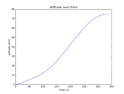
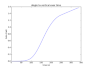
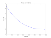
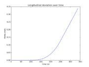
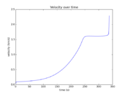
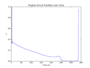
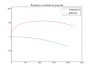
The reference solution was generated using a direct multiple shooting approach with 300 shooting intervals placed equidistantly along the variable-length time horizon. The resulting NLP was implemented using CasADi 2.4.2 using CVodes as an integrator and IPOPT as a solver. The exact code used to solve the problem alongside detailed solution data can be found under Gravity Turn Maneuver (Casadi). The solution achieves the desired orbit in $T = 338.042 \; s$ spending $m_0 - m(T) = 9.6508 \; t$ of fuel. The launch angle is approximately $\beta(0) = 2.7786081986275378 \cdot 10^{-6}$ . The downrange motion throughout the entire launch amounts to a change in polar angle of approximately $\theta(T) = 0.3383474346340064 \approx 19.39^{\circ}$ .

Reference solution plots
Vehicle altitude over time.
Angle $\beta$ over time.
Vehicle mass over time.
Angle $\theta$ over time.
Vehicle velocity over time.
Discretized engine control over time.
Resulting vehicle trajectory relative to reference body surface.

Source Code

Model descriptions are available in

Casadi code at Gravity Turn Maneuver (Casadi)

References

There were no citations found in the article.

@@ Line 1: / Line 1: @@
 {{Dimensions
-|nd        = 5
+|nd        = 1
 |nx        = 5
-|nw        = 0
+|nu        = 1
+|nc        = 11
+|nri       = 2
 |nre       = 7
 }}
@@ Line 10: / Line 12: @@
 == Physical description and model derivation ==
-For the purposes of this model, we start with the following ODE system proposed by Culler et. al.:
+For the purposes of this model, we start with the following ODE system proposed by Culler et. al. in <bib id="Culler1957" />:
 <dd>
@@ Line 93: / Line 95: @@
 </dd>
-Note that if the vehicle is axially symmetric and oriented for its symmetry axis to be parallel to the velocity vector, it does not experience any lift forces. This model is simplified. It does not account for changes in temperature and atmospheric composition with altitude. Also, <math>c_d</math> varies with fluid viscosity and vehicle velocity. Specifically, drastic changes in <math>c_d</math> occur as the vehicle breaks the sound barrier. This is not accounted for in this model.
+Note that if the vehicle is axially symmetric and oriented in such a way that its symmetry axis is parallel to the velocity vector, it does not experience any lift forces. This model is simplified. It does not account for changes in temperature and atmospheric composition with altitude. Also, <math>c_d</math> varies with fluid viscosity and vehicle velocity. Specifically, drastic changes in <math>c_d</math> occur as the vehicle breaks the sound barrier. This is not accounted for in this model.
 == Mathematical formulation ==
@@ Line 102: / Line 104: @@
 <math>
 \begin{array}{llcll}
-  \displaystyle \min_{T, m, v, q, h, d, u} & m_0 - m(T)   \\[1.5ex]
+  \displaystyle \min_{T, m, v, \beta, h, \theta, u} & m_0 - m(T)   \\[1.5ex]
-  \mbox{s.t.} & \dot{x}_0(t) & = & x_0(t) - x_0(t) x_1(t) - \; c_0 x_0(t) \; w(t) \\
+  \mbox{s.t.} & \dot{m} & = & -\frac{F_{max}}{I_{sp} \cdot g_0} \cdot u ,\\
- & \dot{m}(t) & = & -\frac{F_{max}}{I_{sp} \cdot g_0} \cdot u(t) \qquad & \forall t \in [0,T]  \\
+  & \dot{v} & = & (F - \frac{1}{2} \rho_0 \cdot e^{-\frac{h}{H}} A c_d v^2) \cdot \frac{1}{m} - g_0 \cdot \left(\frac{r_0}{r_0 + h}\right)^2 \cos \beta ,\\
-  & \dot{v}(t) & = & \frac{F - \frac{1}{2} \rho_0 \cdot e^{-\frac{h(t)}{H}} A c_d v^2(t)}{m} - g_0 \cdot \left(\frac{r_0}{r_0 + h(t)}\right)^2 \cos \beta(t) \qquad & \forall t \in [0,T]  \\
+  & \dot{\beta} & = & g_0 \cdot \left(\frac{r_0}{r_0 + h}\right)^2 \cdot \frac{\sin{\beta}}{v} - \frac{v \cdot \sin \beta}{r_0 + h} ,\\
-  & \dot{\beta}(t) & = & g_0 \cdot \left(\frac{r_0}{r_0 + h(t)}\right)^2 \cdot \frac{\sin{\beta(t)}}{v(t)} - \frac{v(t) \cdot \sin \beta(t)}{r_0 + h(t)} \qquad & \forall t \in [0,T] \\
+  & \dot{h} & = & v \cdot \cos \beta ,\\
-  & \dot{h}(t) & = & v(t) \cdot \cos \beta(t) \qquad & \forall t \in [0,T] \\
+  & \dot{\theta} & = & \frac{v \cdot \sin \beta}{r_0 + h},\\[1.5ex]
-  & \dot{\theta}(t) & = & \frac{v(t) \cdot \sin \beta(t)}{r_0 + h(t)} \qquad & \forall t \in [0,T] \\[1.5ex]
+  & m(0) &=& m_0 , \\
-  & m(0) &=& m_0 \\
+  & v(0) &=& \varepsilon , \\
-  & v(0) &=& \varepsilon \\
   & \beta(0) &\in& \left[ 0,\frac{\pi}{2} \right], \\
   & h(0) &=& 0, \\
   & \theta(0) &=& 0, \\[1.5ex]
-  & \beta(T) &=& \hat{\beta} \\
+  & \beta(T) &=& \hat{\beta} , \\
-  & h(T) &=& \hat{h} \\
+  & h(T) &=& \hat{h} , \\
-  & v(T) &=& \hat{v} \\[1.5ex]
+  & v(T) &=& \hat{v} , \\[1.5ex]
-  & m(t) &\in& [m_1, m_0] \qquad & \forall t \in [0,T] \\
+  & m(t) &\in& [m_1, m_0] \qquad & \forall t \in [0,T] , \\
-  & v(t) &\geq& \varepsilon \qquad & \forall t \in [0,T] \\
+  & v(t) &\geq& \varepsilon \qquad & \forall t \in [0,T] , \\
-  & \beta(t) &\in& [0, \pi] \qquad & \forall t \in [0,T] \\
+  & \beta(t) &\in& [0, \pi] \qquad & \forall t \in [0,T] , \\
-  & h(t) &\geq& 0 \qquad & \forall t \in [0,T] \\
+  & h(t) &\geq& 0 \qquad & \forall t \in [0,T] , \\
-  & \theta(t) &\geq& 0 \qquad & \forall t \in [0,T] \\[1.5ex]
+  & \theta(t) &\geq& 0 \qquad & \forall t \in [0,T] , \\[1.5ex]
-  & u(t) &\in& [0,1] \qquad & \forall t \in [0,T] \\
+  & u(t) &\in& [0,1] \qquad & \forall t \in [0,T] , \\
   & T &\in& [T_{min}, T_{max}].
 \end{array}
@@ Line 128: / Line 129: @@
 </dd>
 where <math>F_{max}</math> is the maximum thrust of the vehicle's engine and <math>\varepsilon</math> is a small number that is strictly greater than zero.
+The differential states of the problem are <math> m, v, \beta, h, \theta </math> while <math> u </math> is the control function
 == Parameters ==
@@ Line 160: / Line 162: @@
 == Reference solution ==
-(There is currently no reference solution data.)
+The reference solution was generated using a direct multiple shooting approach with 300 shooting intervals placed equidistantly along the variable-length time horizon. The resulting NLP was implemented using CasADi 2.4.2 using CVodes as an integrator and IPOPT as a solver. The exact code used to solve the problem alongside detailed solution data can be found under [[Gravity Turn Maneuver (Casadi)]]. The solution achieves the desired orbit in <math>T = 338.042 \; s</math> spending <math>m_0 - m(T) = 9.6508 \; t</math> of fuel. The launch angle is approximately <math>\beta(0) = 2.7786081986275378 \cdot 10^{-6}</math>. The downrange motion throughout the entire launch amounts to a change in polar angle of approximately <math>\theta(T) = 0.3383474346340064 \approx 19.39^{\circ}</math>.
+<gallery caption="Reference solution plots" widths="180px" heights="140px" perrow="2">
+ Image:gravity-turn-altitude.png| Vehicle altitude over time.
+ Image:gravity-turn-beta.png| Angle <math>\beta</math> over time.
+ Image:gravity-turn-mass.png| Vehicle mass over time.
+ Image:gravity-turn-theta.png| Angle <math>\theta</math> over time.
+ Image:gravity-turn-velocity.png| Vehicle velocity over time.
+ Image:gravity-turn-control.png| Discretized engine control over time.
+ Image:gravity-turn-trajectory.png| Resulting vehicle trajectory relative to reference body surface.
+</gallery>
 == Source Code ==
@@ Line 169: / Line 181: @@
 == References ==
+<biblist />
- CULLER, Glen J.; FRIED, Burton D. Universal gravity turn trajectories. Journal of Applied Physics, 1957, 28. Jg., Nr. 6, S. 672-676.
 <!--List of all categories this page is part of. List characterization of solution behavior, model properties, ore presence of implementation details (e.g., AMPL for AMPL model) here -->
 [[Category:MIOCP]]
 [[Category:ODE model]]
+[[Category:Aeronautics]]
+[[Category:Path-constrained arcs]]

Difference between revisions of "Gravity Turn Maneuver"

Latest revision as of 09:29, 27 July 2016

Contents

Physical description and model derivation

Changes in gravitational acceleration

Decrease in vehicle mass

Curvature of the reference body's surface

Atmospheric drag

Mathematical formulation

Parameters

Reference solution

Source Code

References

Navigation menu

Personal tools

Namespaces

Variants

Views

More

Search

Navigation

Support

Tools