Difference between revisions of "F-8 aircraft"

F-8 aircraft
State dimension:	1
Differential states:	3
Discrete control functions:	1
Interior point equalities:	6

Revision as of 17:39, 9 July 2009

The F-8 aircraft control problem is based on a very simple aircraft model. The control problem was introduced by Kaya and Noakes and aims at controlling an aircraft in a time-optimal way from an initial state to a terminal state.

The mathematical equations form a small-scale ODE model. The interior point equality conditions fix both initial and terminal values of the differential states.

The optimal, relaxed control function shows bang bang behavior. The problem is furthermore interesting as it should be reformulated equivalently.

Mathematical formulation

For $t \in [0, T]$ almost everywhere the mixed-integer optimal control problem is given by

$\begin{array}{llcl} \displaystyle \min_{x, w, T} & T \\[1.5ex] \mbox{s.t.} & \dot{x}_0 &=& -0.877 \; x_0 + x_2 - 0.088 \; x_0 \; x_2 + 0.47 \; x_0^2 - 0.019 \; x_1^2 - x_0^2 \; x_2 + 3.846 \; x_0^3 \\ &&& - 0.215 \; w + 0.28 \; x_0^2 \; w + 0.47 \; x_0 \; w^2 + 0.63 \; w^3 \\ & \dot{x}_1 &=& x_2 \\ & \dot{x}_2 &=& -4.208 \; x_0 - 0.396 \; x_2 - 0.47 \; x_0^2 - 3.564 \; x_0^3 \\ &&& - 20.967 \; w + 6.265 \; x_0^2 \; w + 46 \; x_0 \; w^2 + 61.4 \; w^3 \\ & x(0) &=& (0.4655,0,0)^T, \\ & x(T) &=& (0,0,0)^T, \\ & w(t) &\in& \{-0.05236,0.05236\}. \end{array}$

$x_0$ is the angle of attack in radians, $x_1$ is the pitch angle, $x_2$ is the pitch rate in rad/s, and the control function $w = w(t)$ is the tail deflection angle in radians. This model goes back to Garrard<bibref>Garrard1977</bibref>.

In the control problem, both initial and terminal values of the differential states are fixed.

Reformulation

The control w(t) is restricted to take values from a finite set only. Hence, the control problem can be reformulated equivalently to

$\begin{array}{llcl} \displaystyle \min_{x, w, T} & T \\[1.5ex] \mbox{s.t.} & \dot{x}_0 &=& -0.877 \; x_0 + x_2 - 0.088 \; x_0 \; x_2 + 0.47 \; x_0^2 - 0.019 \; x_1^2 - x_0^2 \; x_2 + 3.846 \; x_0^3 \\ &&& - \left( 0.215 \; \xi - 0.28 \; x_0^2 \; \xi - 0.47 \; x_0 \; \xi^2 - 0.63 \; \xi^3 \right) \; w \\ &&& - \left( - 0.215 \; \xi + 0.28 \; x_0^2 \; \xi - 0.47 \; x_0 \; \xi^2 + 0.63 \; \xi^3 \right) \; (1 - w) \\ & &=& -0.877 \; x_0 + x_2 - 0.088 \; x_0 \; x_2 + 0.47 \; x_0^2 - 0.019 \; x_1^2 - x_0^2 \; x_2 + 3.846 \; x_0^3 \\ &&& + 0.215 \; \xi - 0.28 \; x_0^2 \; \xi + 0.47 \; x_0 \; \xi^2 - 0.63 \; \xi^3 \\ &&& - \left( 0.215 \; \xi - 0.28 \; x_0^2 \; \xi - 0.63 \; \xi^3 \right) \; 2 w \\ & \dot{x}_1 &=& x_2 \\ & \dot{x}_2 &=& -4.208 \; x_0 - 0.396 \; x_2 - 0.47 \; x_0^2 - 3.564 \; x_0^3 \\ &&& - \left( 20.967 \; \xi - 6.265 \; x_0^2 \; \xi -46 \; x_0 \; \xi^2 - 61.4 \; \xi^3 \right) \; w \\ &&& - \left( - 20.967 \; \xi + 6.265 \; x_0^2 \; \xi -46 \; x_0 \; \xi^2 + 61.4 \; \xi^3 \right) \; (1 - w) \\ & &=& -4.208 \; x_0 - 0.396 \; x_2 - 0.47 \; x_0^2 - 3.564 \; x_0^3 \\ &&& + 20.967 \; \xi - 6.265 \; x_0^2 \; \xi + 46 \; x_0 \; \xi^2 - 61.4 \; \xi^3 \\ &&& - \left( 20.967 \; \xi - 6.265 \; x_0^2 \; \xi - 61.4 \; \xi^3 \right) \; 2 w \\ & x(0) &=& (0.4655,0,0)^T, \\ & x(T) &=& (0,0,0)^T, \\ & w(t) &\in& \{0,1\}, \end{array}$

with $\xi = 0.05236$ . Note that there is a bijection between optimal solutions of the two problems.

Reference solutions

We provide here a comparison of different solutions reported in the literature. The numbers show the respective lengths $t_i - t_{i-1}$ of the switching arcs with the value of $w(t)$ on the upper or lower bound (given in the second column). Claim denotes what is stated in the respective publication, Simulation shows values obtained by a simulation with a Runge-Kutta-Fehlberg method of 4th/5th order and an integration tolerance of $10^{-8}$ .

Arc	w(t)	Lee et al.<bibref>Lee1997a</bibref>	Kaya<bibref>Kaya2003</bibref>	Sager<bibref>Sager2005</bibref>	Schlueter/ Gerdts	Sager
1	1	0.00000	0.10292	0.10235	0.0	1.13492
2	0	2.18800	1.92793	1.92812	0.608750	0.34703
3	1	0.16400	0.16687	0.16645	3.136514	1.60721
4	0	2.88100	2.74338	2.73071	0.654550	0.69169
5	1	0.33000	0.32992	0.32994	0.0	0.0
6	0	0.47200	0.47116	0.47107	0.0	0.0
Claim: Infeasibility	-	1.00E-10	7.30E-06	5.90E-06	3.29169e-06	2.21723e-07
Claim: Objective	-	6.03500	5.74217	5.72864	4.39981	3.78086
Simulation: Infeasibility	-	1.75E-03	1.64E-03	5.90E-06	3.29169e-06	2.21723e-07
Simulation: Objective	-	6.03500	5.74218	5.72864	4.39981	3.78086

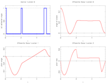
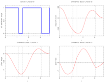
The best known optimal objective value of this problem given is given by 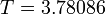$T = 3.78086$ . The corresponding solution is shown in the rightmost plot. The solution of bang-bang type switches three times, starting with $w(t) = 1$ .

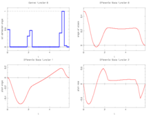
Reference solution plots
Locally optimal relaxed control on a coarse control discretization grid and corresponding differential states.
Locally optimal relaxed control on a fine, adaptively chosen control discretization grid and corresponding differential states.
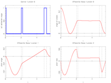
Integer control and corresponding differential states from Sager<bibref>Sager2005</bibref>.
Integer control and corresponding differential states from Schlueter/ Gerdts solution.
Best known integer control and corresponding differential states from Sager solution.

Source Code

C

The differential equations in C code:

  double x1 = xd[0];
  double x2 = xd[1];
  double x3 = xd[2];
 
#ifdef CONVEXIFIED
  double xi = 0.05236;
 
  rhs[0] = -0.877*x1 + x3 - 0.088*x1*x3 + 0.47*x1*x1 - 0.019*x2*x2 -x1*x1*x3 + 3.846*x1*x1*x1
	         + 0.215*xi - 0.28*x1*x1*xi + 0.47*x1*xi*xi - 0.63*xi*xi*xi
	         - 2*u[0] * ( 0.215*xi - 0.28*x1*x1*xi - 0.63*xi*xi*xi );
  rhs[1] = x3;
  rhs[2] = - 4.208*x1 - 0.396*x3 - 0.47*x1*x1 - 3.564*x1*x1*x1
	         + 20.967*xi - 6.265*x1*x1*xi + 46*x1*xi*xi - 61.4*xi*xi*xi
	         - 2*u[0] * ( 20.967*xi - 6.265*x1*x1*xi - 61.4*xi*xi*xi );
#else
  double u_ = -0.05236 + u[0]*2.0*0.05236;
 
  rhs[0] = -0.877*x1 + x3 - 0.088*x1*x3 + 0.47*x1*x1 - 0.019*x2*x2
           -x1*x1*x3 + 3.846*x1*x1*x1 - 0.215*u_ + 0.28*x1*x1*u_ + 0.47*x1*u_*u_ + 0.63*u_*u_*u_;
  rhs[1] = x3;
  rhs[2] = -4.208*x1 - 0.396*x3 - 0.47*x1*x1 - 3.564*x1*x1*x1
           - 20.967*u_ + 6.265*x1*x1*u_ + 46*x1*u_*u_ + 61.4*u_*u_*u_;
#endif

Variants

a prescribed time grid for the control function, see F-8 aircraft (AMPL),

Miscellaneous and Further Reading

See <bibref>Kaya2003</bibref> and <bibref>Sager2005</bibref> for details.

References

@@ Line 133: / Line 133: @@
 </source>
+== Variants ==
+* a prescribed time grid for the control function, see [[F-8 aircraft (AMPL)]],
 == Miscellaneous and Further Reading ==

Difference between revisions of "F-8 aircraft"

Revision as of 17:39, 9 July 2009

Contents

Mathematical formulation

Reformulation

Reference solutions

Source Code

C

Variants

Miscellaneous and Further Reading

References

Navigation menu

Personal tools

Namespaces

Variants

Views

More

Search

Navigation

Support

Tools