Difference between revisions of "F-8 aircraft"
m (Added plots) |
FelixMueller (Talk | contribs) |
||
| (32 intermediate revisions by 7 users not shown) | |||
| Line 3: | Line 3: | ||
|nx = 3 | |nx = 3 | ||
|nw = 1 | |nw = 1 | ||
| + | |nc = 2 | ||
|nre = 6 | |nre = 6 | ||
}} | }} | ||
| − | The F-8 aircraft control problem is based on a very simple aircraft model. The control problem was introduced by Kaya and Noakes | + | The F-8 aircraft control problem is based on a very simple aircraft model. The control problem was introduced by Kaya and Noakes and aims at controlling an aircraft in a time-optimal way from an initial state to a terminal state. |
| − | The mathematical equations form a small-scale [[:Category:ODE | + | The mathematical equations form a small-scale [[:Category:ODE model|ODE model]]. The interior point equality conditions fix both initial and terminal values of the differential states. |
| − | The optimal | + | The optimal, relaxed control function shows [[:Category:Bang bang|bang bang]] behavior. The problem is furthermore interesting as it should be reformulated equivalently. |
== Mathematical formulation == | == Mathematical formulation == | ||
| Line 19: | Line 20: | ||
\begin{array}{llcl} | \begin{array}{llcl} | ||
\displaystyle \min_{x, w, T} & T \\[1.5ex] | \displaystyle \min_{x, w, T} & T \\[1.5ex] | ||
| − | \mbox{s.t.} & \dot{x}_0 &=& -0.877 \; x_0 + x_2 - 0.088 \; x_0 \; x_2 + 0.47 \; x_0^2 - 0.019 \; x_1^2 - x_0^2 \; x_2 | + | \mbox{s.t.} & \dot{x}_0 &=& -0.877 \; x_0 + x_2 - 0.088 \; x_0 \; x_2 + 0.47 \; x_0^2 - 0.019 \; x_1^2 - x_0^2 \; x_2 + 3.846 \; x_0^3 \\ |
| − | + | &&& - 0.215 \; w + 0.28 \; x_0^2 \; w + 0.47 \; x_0 \; w^2 + 0.63 \; w^3 \\ | |
& \dot{x}_1 &=& x_2 \\ | & \dot{x}_1 &=& x_2 \\ | ||
& \dot{x}_2 &=& -4.208 \; x_0 - 0.396 \; x_2 - 0.47 \; x_0^2 - 3.564 \; x_0^3 \\ | & \dot{x}_2 &=& -4.208 \; x_0 - 0.396 \; x_2 - 0.47 \; x_0^2 - 3.564 \; x_0^3 \\ | ||
| − | & x(0) &=& | + | &&& - 20.967 \; w + 6.265 \; x_0^2 \; w + 46 \; x_0 \; w^2 + 61.4 \; w^3 \\ |
| − | & x(T) &=& | + | & x(0) &=& (0.4655,0,0)^T, \\ |
| + | & x(T) &=& (0,0,0)^T, \\ | ||
& w(t) &\in& \{-0.05236,0.05236\}. | & w(t) &\in& \{-0.05236,0.05236\}. | ||
\end{array} | \end{array} | ||
</math> | </math> | ||
| − | <math>x_0</math> is the angle of attack in radians, <math>x_1</math> is the pitch angle, <math>x_2</math> is the pitch rate in rad/s, and the control function <math>w = w(t)</math> is the tail deflection angle in radians. This model goes back to Garrard< | + | <math>x_0</math> is the angle of attack in radians, <math>x_1</math> is the pitch angle, <math>x_2</math> is the pitch rate in rad/s, and the control function <math>w = w(t)</math> is the tail deflection angle in radians. This model goes back to Garrard<bib id="Garrard1977" />. |
| − | + | In the control problem, both initial and terminal values of the differential states are fixed. | |
| − | == | + | == Reformulation == |
| − | + | The control w(t) is restricted to take values from a finite set only. Hence, the control problem can be reformulated equivalently to | |
<math> | <math> | ||
| − | \begin{array}{ | + | \begin{array}{llcl} |
| − | x_0 &=& (0.4655,0,0)^T, \\ | + | \displaystyle \min_{x, w, T} & T \\[1.5ex] |
| − | + | \mbox{s.t.} & \dot{x}_0 &=& -0.877 \; x_0 + x_2 - 0.088 \; x_0 \; x_2 + 0.47 \; x_0^2 - 0.019 \; x_1^2 - x_0^2 \; x_2 + 3.846 \; x_0^3 \\ | |
| − | \end{array} | + | &&& - \left( 0.215 \; \xi - 0.28 \; x_0^2 \; \xi - 0.47 \; x_0 \; \xi^2 - 0.63 \; \xi^3 \right) \; w \\ |
| + | &&& - \left( - 0.215 \; \xi + 0.28 \; x_0^2 \; \xi - 0.47 \; x_0 \; \xi^2 + 0.63 \; \xi^3 \right) \; (1 - w) \\ | ||
| + | & &=& -0.877 \; x_0 + x_2 - 0.088 \; x_0 \; x_2 + 0.47 \; x_0^2 - 0.019 \; x_1^2 - x_0^2 \; x_2 + 3.846 \; x_0^3 \\ | ||
| + | &&& + 0.215 \; \xi - 0.28 \; x_0^2 \; \xi + 0.47 \; x_0 \; \xi^2 - 0.63 \; \xi^3 \\ | ||
| + | &&& - \left( 0.215 \; \xi - 0.28 \; x_0^2 \; \xi - 0.63 \; \xi^3 \right) \; 2 w \\ | ||
| + | & \dot{x}_1 &=& x_2 \\ | ||
| + | & \dot{x}_2 &=& -4.208 \; x_0 - 0.396 \; x_2 - 0.47 \; x_0^2 - 3.564 \; x_0^3 \\ | ||
| + | &&& - \left( 20.967 \; \xi - 6.265 \; x_0^2 \; \xi -46 \; x_0 \; \xi^2 - 61.4 \; \xi^3 \right) \; w \\ | ||
| + | &&& - \left( - 20.967 \; \xi + 6.265 \; x_0^2 \; \xi -46 \; x_0 \; \xi^2 + 61.4 \; \xi^3 \right) \; (1 - w) \\ | ||
| + | & &=& -4.208 \; x_0 - 0.396 \; x_2 - 0.47 \; x_0^2 - 3.564 \; x_0^3 \\ | ||
| + | &&& + 20.967 \; \xi - 6.265 \; x_0^2 \; \xi + 46 \; x_0 \; \xi^2 - 61.4 \; \xi^3 \\ | ||
| + | &&& - \left( 20.967 \; \xi - 6.265 \; x_0^2 \; \xi - 61.4 \; \xi^3 \right) \; 2 w \\ | ||
| + | & x(0) &=& (0.4655,0,0)^T, \\ | ||
| + | & x(T) &=& (0,0,0)^T, \\ | ||
| + | & w(t) &\in& \{0,1\}, | ||
| + | \end{array} | ||
</math> | </math> | ||
| + | |||
| + | with <math>\xi = 0.05236</math>. Note that there is a bijection between optimal solutions of the two problems. | ||
== Reference solutions == | == Reference solutions == | ||
| − | + | We provide here a comparison of different solutions reported in the literature. The numbers show the respective lengths <math>t_i - t_{i-1}</math> of the switching arcs with the value of <math>w(t)</math> on the upper or lower bound (given in the second column). ''Claim'' denotes what is stated in the respective publication, ''Simulation'' shows values obtained by a simulation with a Runge-Kutta-Fehlberg method of 4th/5th order and an integration tolerance of <math>10^{-8}</math>. | |
| + | {| border="1" align="center" cellpadding="5" cellspacing="0" | ||
| + | |- bgcolor=#c7c7c7 | ||
| + | ! Arc !! w(t) !! Lee et al.<bib id="Lee1997a" /> !! Kaya<bib id="Kaya2003" /> !! Sager<bib id="Sager2005" /> !! [[User:MartinSchlueter | Schlueter]]/[[User:Matthias.gerdts | Gerdts]] !! Sager | ||
| + | |- | ||
| + | | align=center | 1 || align=center | 1 || 0.00000 || 0.10292 || 0.10235 || 0.0 || 1.13492 | ||
| + | |- | ||
| + | | align=center | 2 || align=center | 0 || 2.18800 || 1.92793 || 1.92812 || 0.608750 || 0.34703 | ||
| + | |- | ||
| + | | align=center | 3 || align=center | 1 || 0.16400 || 0.16687 || 0.16645 || 3.136514 || 1.60721 | ||
| + | |- | ||
| + | | align=center | 4 || align=center | 0 || 2.88100 || 2.74338 || 2.73071 || 0.654550 || 0.69169 | ||
| + | |- | ||
| + | | align=center | 5 || align=center | 1 || 0.33000 || 0.32992 || 0.32994 || 0.0 || 0.0 | ||
| + | |- | ||
| + | | align=center | 6 || align=center | 0 || 0.47200 || 0.47116 || 0.47107 || 0.0 || 0.0 | ||
| + | |- | ||
| + | | Claim: Infeasibility || align=center | - || 1.00E-10 || 7.30E-06 || 5.90E-06 || 3.29169e-06 || 2.21723e-07 | ||
| + | |- | ||
| + | | Claim: Objective || align=center | - || 6.03500 || 5.74217 || 5.72864 || 4.39981 || 3.78086 | ||
| + | |- style="font-style:italic;background-color:#ffffcc;" | ||
| + | ! Simulation: Infeasibility || align=center | - || 1.75E-03 || 1.64E-03 || 5.90E-06 || 3.29169e-06 || 2.21723e-07 | ||
| + | |- style="font-style:italic;background-color:#ffffcc;" | ||
| + | ! Simulation: Objective || align=center | - || 6.03500 || 5.74218 || 5.72864 || 4.39981 || 3.78086 | ||
| + | |} | ||
| + | |||
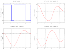
| + | The best known optimal objective value of this problem given is given by <math>T = 3.78086</math>. The corresponding solution is shown in the rightmost plot. The solution of bang-bang type switches three times, starting with <math>w(t) = 1</math>. | ||
| + | |||
<gallery caption="Reference solution plots" widths="240px" heights="167px" perrow="3"> | <gallery caption="Reference solution plots" widths="240px" heights="167px" perrow="3"> | ||
| − | Image:f8aircraftRelaxedCoarse.png| | + | Image:f8aircraftRelaxedCoarse.png| Locally optimal relaxed control on a coarse control discretization grid and corresponding differential states. |
| − | Image:f8aircraftRelaxedFine.png| | + | Image:f8aircraftRelaxedFine.png| Locally optimal relaxed control on a fine, adaptively chosen control discretization grid and corresponding differential states. |
| − | Image:f8aircraftInteger.png| | + | Image:f8aircraftInteger.png| Integer control and corresponding differential states from Sager<bib id="Sager2005" />. |
| + | |||
| + | Image:f8aircraftSchlueter.png| Integer control and corresponding differential states from [[User:MartinSchlueter | Schlueter]]/[[User:Matthias.gerdts | Gerdts]] solution. | ||
| + | Image:f8aircraftSager2009.png| Best known integer control and corresponding differential states from Sager solution. | ||
</gallery> | </gallery> | ||
| − | == | + | === jModelica === |
| − | === | + | Objective : 5.12799232 |
| + | infeasibility : 6.2235588037251599e-10 | ||
| + | |||
| + | <gallery caption="Obtained solution plots" widths="240px" heights="167px" perrow="3"> | ||
| + | Image:f8aircraft1.png| (Probably sub-)Optimal control. | ||
| + | Image:f8aircraft2.png| Corresponding differential states. | ||
| + | |||
| + | </gallery> | ||
| + | |||
| + | == Source Code == | ||
| − | + | Model descriptions are available in | |
| − | + | ||
| − | + | ||
| − | + | ||
| − | + | ||
| − | + | * [[:Category:AMPL | AMPL code]] at [[F-8 aircraft (AMPL)]] | |
| − | + | * [[:Category:Muscod | Muscod code]] at [[F-8 aircraft (Muscod)]] | |
| − | + | * [[:Category:JModelica | JModelica code]] at [[F-8 aircraft (JModelica)]] | |
| − | + | ||
| − | + | ||
| − | + | ||
| − | + | ||
| − | + | ||
| − | + | ||
| − | + | ||
| − | + | == Variants == | |
| − | + | ||
| − | + | ||
| − | + | ||
| − | + | ||
| − | + | * a prescribed time grid for the control function, see [[F-8 aircraft (AMPL)]], | |
| − | + | ||
| − | + | ||
| − | + | ||
== Miscellaneous and Further Reading == | == Miscellaneous and Further Reading == | ||
| − | See < | + | See <bib id="Kaya2003" /> and <bib id="Sager2005" /> for details. |
== References == | == References == | ||
| − | < | + | <biblist /> |
<!--List of all categories this page is part of. List characterization of solution behavior, model properties, ore presence of implementation details (e.g., AMPL for AMPL model) here --> | <!--List of all categories this page is part of. List characterization of solution behavior, model properties, ore presence of implementation details (e.g., AMPL for AMPL model) here --> | ||
[[Category:Bang bang]] | [[Category:Bang bang]] | ||
[[Category:MIOCP]] | [[Category:MIOCP]] | ||
| − | [[Category:ODE | + | [[Category:ODE model]] |
| + | [[Category:Aeronautics]] | ||
| + | [[Category:Outer convexification]] | ||
| + | [[Category: Minimum time]] | ||
Latest revision as of 10:29, 27 July 2016
| F-8 aircraft | |
|---|---|
| State dimension: | 1 |
| Differential states: | 3 |
| Discrete control functions: | 1 |
| Path constraints: | 2 |
| Interior point equalities: | 6 |
The F-8 aircraft control problem is based on a very simple aircraft model. The control problem was introduced by Kaya and Noakes and aims at controlling an aircraft in a time-optimal way from an initial state to a terminal state.
The mathematical equations form a small-scale ODE model. The interior point equality conditions fix both initial and terminal values of the differential states.
The optimal, relaxed control function shows bang bang behavior. The problem is furthermore interesting as it should be reformulated equivalently.
Contents
Mathematical formulation
For ![t \in [0, T]](https://mintoc.de/images/math/e/6/6/e66a2b7fedcba80ccb192b87440f8d9c.png) almost everywhere the mixed-integer optimal control problem is given by
almost everywhere the mixed-integer optimal control problem is given by
![\begin{array}{llcl}
\displaystyle \min_{x, w, T} & T \\[1.5ex]
\mbox{s.t.} & \dot{x}_0 &=& -0.877 \; x_0 + x_2 - 0.088 \; x_0 \; x_2 + 0.47 \; x_0^2 - 0.019 \; x_1^2 - x_0^2 \; x_2 + 3.846 \; x_0^3 \\
&&& - 0.215 \; w + 0.28 \; x_0^2 \; w + 0.47 \; x_0 \; w^2 + 0.63 \; w^3 \\
& \dot{x}_1 &=& x_2 \\
& \dot{x}_2 &=& -4.208 \; x_0 - 0.396 \; x_2 - 0.47 \; x_0^2 - 3.564 \; x_0^3 \\
&&& - 20.967 \; w + 6.265 \; x_0^2 \; w + 46 \; x_0 \; w^2 + 61.4 \; w^3 \\
& x(0) &=& (0.4655,0,0)^T, \\
& x(T) &=& (0,0,0)^T, \\
& w(t) &\in& \{-0.05236,0.05236\}.
\end{array}](https://mintoc.de/images/math/d/2/b/d2bd7e6d1cc8affb72d59248a105d528.png)
 is the angle of attack in radians,
  is the pitch angle,
  is the pitch rate in rad/s, and the control function
  is the tail deflection angle in radians. This model goes back to Garrard[Garrard1977]Author: Garrard, W.L.; Jordan, J.M.
Journal: Automatica
Pages: 497--505
Title: Design of Nonlinear Automatic Control Systems
Volume: 13
Year: 1977 .
.
In the control problem, both initial and terminal values of the differential states are fixed.
Reformulation
The control w(t) is restricted to take values from a finite set only. Hence, the control problem can be reformulated equivalently to
![\begin{array}{llcl}
\displaystyle \min_{x, w, T} & T \\[1.5ex]
\mbox{s.t.} & \dot{x}_0 &=& -0.877 \; x_0 + x_2 - 0.088 \; x_0 \; x_2 + 0.47 \; x_0^2 - 0.019 \; x_1^2 - x_0^2 \; x_2 + 3.846 \; x_0^3 \\
&&& - \left( 0.215 \; \xi - 0.28 \; x_0^2 \; \xi - 0.47 \; x_0 \; \xi^2 - 0.63 \; \xi^3 \right) \; w \\
&&& - \left( - 0.215 \; \xi + 0.28 \; x_0^2 \; \xi - 0.47 \; x_0 \; \xi^2 + 0.63 \; \xi^3 \right) \; (1 - w) \\
& &=& -0.877 \; x_0 + x_2 - 0.088 \; x_0 \; x_2 + 0.47 \; x_0^2 - 0.019 \; x_1^2 - x_0^2 \; x_2 + 3.846 \; x_0^3 \\
&&& + 0.215 \; \xi - 0.28 \; x_0^2 \; \xi + 0.47 \; x_0 \; \xi^2 - 0.63 \; \xi^3 \\
&&& - \left( 0.215 \; \xi - 0.28 \; x_0^2 \; \xi - 0.63 \; \xi^3 \right) \; 2 w \\
& \dot{x}_1 &=& x_2 \\
& \dot{x}_2 &=& -4.208 \; x_0 - 0.396 \; x_2 - 0.47 \; x_0^2 - 3.564 \; x_0^3 \\
&&& - \left( 20.967 \; \xi - 6.265 \; x_0^2 \; \xi -46 \; x_0 \; \xi^2 - 61.4 \; \xi^3 \right) \; w \\
&&& - \left( - 20.967 \; \xi + 6.265 \; x_0^2 \; \xi -46 \; x_0 \; \xi^2 + 61.4 \; \xi^3 \right) \; (1 - w) \\
& &=& -4.208 \; x_0 - 0.396 \; x_2 - 0.47 \; x_0^2 - 3.564 \; x_0^3 \\
&&& + 20.967 \; \xi - 6.265 \; x_0^2 \; \xi + 46 \; x_0 \; \xi^2 - 61.4 \; \xi^3 \\
&&& - \left( 20.967 \; \xi - 6.265 \; x_0^2 \; \xi - 61.4 \; \xi^3 \right) \; 2 w \\
& x(0) &=& (0.4655,0,0)^T, \\
& x(T) &=& (0,0,0)^T, \\
& w(t) &\in& \{0,1\},
\end{array}](https://mintoc.de/images/math/0/4/a/04a0e56e2d185c764c658785ce00ade8.png)
with  . Note that there is a bijection between optimal solutions of the two problems.
Reference solutions
We provide here a comparison of different solutions reported in the literature. The numbers show the respective lengths  of the switching arcs with the value of
  on the upper or lower bound (given in the second column). Claim denotes what is stated in the respective publication, Simulation shows values obtained by a simulation with a Runge-Kutta-Fehlberg method of 4th/5th order and an integration tolerance of
  .
.
| Arc | w(t) | Lee et al.[Lee1997a]Author: Lee, H.W.J.; Teo, K.L.; Rehbock, V.; Jennings, L.S. Journal: Dynamic Systems and Applications Pages: 243--262 Title: Control Parametrization Enhancing Technique for Time-Optimal Control Problems Volume: 6 Year: 1997 |
Kaya[Kaya2003]Author: C.Y. Kaya; J.L. Noakes Journal: Journal of Optimization Theory and Applications Pages: 69--92 Title: A Computational Method for Time-Optimal Control Volume: 117 Year: 2003 |
Sager[Sager2005]Address: Tönning, Lübeck, Marburg Author: S. Sager Editor: ISBN 3-89959-416-9 Publisher: Der andere Verlag Title: Numerical methods for mixed--integer optimal control problems Url: http://mathopt.de/PUBLICATIONS/Sager2005.pdf Year: 2005 |
Schlueter/ Gerdts | Sager |
|---|---|---|---|---|---|---|
| 1 | 1 | 0.00000 | 0.10292 | 0.10235 | 0.0 | 1.13492 |
| 2 | 0 | 2.18800 | 1.92793 | 1.92812 | 0.608750 | 0.34703 |
| 3 | 1 | 0.16400 | 0.16687 | 0.16645 | 3.136514 | 1.60721 |
| 4 | 0 | 2.88100 | 2.74338 | 2.73071 | 0.654550 | 0.69169 |
| 5 | 1 | 0.33000 | 0.32992 | 0.32994 | 0.0 | 0.0 |
| 6 | 0 | 0.47200 | 0.47116 | 0.47107 | 0.0 | 0.0 |
| Claim: Infeasibility | - | 1.00E-10 | 7.30E-06 | 5.90E-06 | 3.29169e-06 | 2.21723e-07 |
| Claim: Objective | - | 6.03500 | 5.74217 | 5.72864 | 4.39981 | 3.78086 |
| Simulation: Infeasibility | - | 1.75E-03 | 1.64E-03 | 5.90E-06 | 3.29169e-06 | 2.21723e-07 |
| Simulation: Objective | - | 6.03500 | 5.74218 | 5.72864 | 4.39981 | 3.78086 |
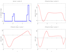
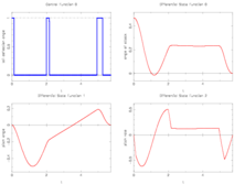
The best known optimal objective value of this problem given is given by  . The corresponding solution is shown in the rightmost plot. The solution of bang-bang type switches three times, starting with
  .
.
- Reference solution plots
Locally optimal relaxed control on a coarse control discretization grid and corresponding differential states.
Locally optimal relaxed control on a fine, adaptively chosen control discretization grid and corresponding differential states.
Integer control and corresponding differential states from Sager[Sager2005]Address: Tönning, Lübeck, Marburg
Author: S. Sager
Editor: ISBN 3-89959-416-9
Publisher: Der andere Verlag
Title: Numerical methods for mixed--integer optimal control problems
Url: http://mathopt.de/PUBLICATIONS/Sager2005.pdf
Year: 2005.
Best known integer control and corresponding differential states from Sager solution.


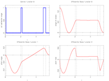
jModelica
Objective : 5.12799232 infeasibility : 6.2235588037251599e-10
- Obtained solution plots
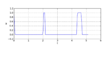
(Probably sub-)Optimal control.
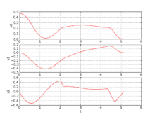
Corresponding differential states.


Source Code
Model descriptions are available in
- AMPL code at F-8 aircraft (AMPL)
- Muscod code at F-8 aircraft (Muscod)
- JModelica code at F-8 aircraft (JModelica)
Variants
- a prescribed time grid for the control function, see F-8 aircraft (AMPL),
Miscellaneous and Further Reading
See [Kaya2003]Author: C.Y. Kaya; J.L. Noakes
Journal: Journal of Optimization Theory and Applications
Pages: 69--92
Title: A Computational Method for Time-Optimal Control
Volume: 117
Year: 2003 and [Sager2005]Address: Tönning, Lübeck, Marburg
Author: S. Sager
Editor: ISBN 3-89959-416-9
Publisher: Der andere Verlag
Title: Numerical methods for mixed--integer optimal control problems
Url: http://mathopt.de/PUBLICATIONS/Sager2005.pdf
Year: 2005 for details.
References
There were no citations found in the article.