Source Inversion
The source inversion problem is a very basic problem in mixed-integer PDE constrained optimization. It has one PDE constraint equivalent to an inhomogenous Poisson problem with Robin-type boundary conditions. This type of problem arises naturally from the task of finding stationary solutions to the heat equation where the problem domain represents a medium being either heated or cooled and heat is lost to a surrounding medium at a rate proportional to the difference between the temperatures of the domain boundary and the surrounding medium.
The right hand side of Poisson's equation is sometimes referred to as the source term. For the purposes of the source inversion problem, the source term is assumed to be a linear combination of a finite set of predefined terms with coefficients being chosen from  . The objective is to find a source term such that the solution of the Poisson problem closely tracks a given function over the domain.
Contents
[hide]Problem Statement
For the purposes of this discussion, we will restrict ourselves to a one-dimensional setting and assume that the domain under consideration is the interval ![[0,1]](https://mintoc.de/images/math/c/c/f/ccfcd347d0bf65dc77afe01a3306a96b.png) . The Poisson problem with simple Robin-type boundary conditions then takes the following form:
. The Poisson problem with simple Robin-type boundary conditions then takes the following form:
Here,  denotes the source term. For a more general version of Robin-type boundary conditions, refer to the controlled heating problem which discusses the same problem in a multi-dimensional setting. Given a control grid
 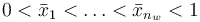 , the elementary source terms are given by:
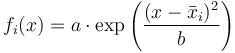
The parameters  and
and  are shared between the individual elementary source terms. Given a reference function
  , the source inversion problem is given by:
![\begin{array}[t]{rl}
\min\limits_{u,w} & \int\limits_0^1 (u - u_d)^2 \, \mathrm{d}x \\
\text{s.t.} & \begin{array}[t]{rll}
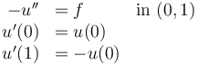
-u'' &= \sum\limits_{i = 1}^{n_w} w_i f_i \qquad &\text{in } (0,1) \\[1.5ex]
u'(0) &= u(0) & \\
u'(1) &= -u(1) & \\[1.5ex]
\sum\limits_{i = 1}^{n_w} w_i &\leq N \\
w_i &\in \lbrace 0, 1 \rbrace \qquad & \forall i \in \lbrace 1, \ldots, n_w \rbrace
\end{array}
\end{array}](https://mintoc.de/images/math/5/6/d/56da072914662fc6073418e13582de83.png)
Weak formulation
Some PDE discretization techniques (such as finite element methods) require the use of weak formulations of the original problem. The weak formulation of the Poisson problem with Robin-type boundary conditions as described above is obtained using Green's identities:
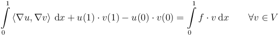
Here,  is a suitable space of test functions. The optimization problem then takes the following form:
![\begin{array}[t]{rl}
\min\limits_{u,w} & \int\limits_0^1 (u - u_d)^2 \, \mathrm{d}x \\
\text{s.t.} & \begin{array}[t]{rll}
\int\limits_0^1 \left\langle \nabla u, \nabla v \right\rangle \,\mathrm{d}x + u(1) \cdot v(1) - u(0) \cdot v(0) &= \sum\limits_{i = 0}^{n_w} \left( w_i \cdot \int\limits_0^1 f_i \cdot v \,\mathrm{d}x \right) \qquad &\forall v \in V \\[1.5ex]
\sum\limits_{i = 1}^{n_w} w_i &\leq N \\
w_i &\in \lbrace 0, 1 \rbrace \qquad & \forall i \in \lbrace 1, \ldots, n_w \rbrace
\end{array}
\end{array}](https://mintoc.de/images/math/4/2/4/424819fbae5d5bdc82178d5621baa246.png)
Parameters
For testing purposes, the following parameters were chosen:
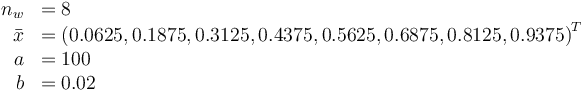
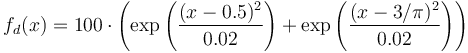
The reference solution is generated as a solution to the Poisson problem using the following source term:
Reference solution
The reference solution was generated using finite element discretizations with an equidistant mesh of  cells. Continuous Galerkin elements of degree
  were employed. The linear FEM system was generated using FEniCS and used as part of the constraints in a QP that was solved using CasADi's IPOPT interface. The integer solution was determined using a simple Branch and Bound algorithm. The exact code used to solve the problem alongside detailed solution data can be found under Source Inversion (FEniCS/Casadi). The optimal objective function value is
  .
.
- Reference solution plots
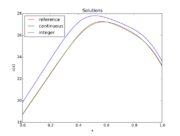
Solutions.
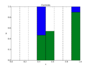
Controls.


Source Code
Model descriptions are available in
- Casadi code using FEniCS at Source Inversion (FEniCS/Casadi)