Direct Current Transmission Heating Problem

Direct Current Transmission Heating Problem
State dimension:	1
Differential states:	3
Discrete control functions:	1
Interior point equalities:	3

The direct current transfer heating problem models a simplified flow of direct electrical current within an electrical network with defined producers and consumers of electrical power. The model includes heating and cooling that occurs in electrical conductors due to specific resistance and heat exchange with the surrounding air. An optimal strategy for regulating the power production of individual producers as well as voltages and currents on specific conductors with the goal of minimizing the net power loss due to heating on all power lines over a fixed time horizon while fully supplying all consumers.

The model is largely assembled from well-known basic descriptions of phenomena easily accessible to the audience of high-school level physics courses. Mainly, these are Ohm's law, electrical resistivity, Joule heating and thermal conductivity. Note that changes of resistivity with temperature are taken into account.

Physical background

The aim of the controller in this model is to provide all consumers with their required amount of electric power. Electric power is given by the product of voltage and current $P = I \cdot U$. The electric power is brought to the consumers from producers via a network of power lines. Producers are assumed to have the capability of accurately regulating their power output within a certain range. Power lines are assumed to be solid blocks of an electrically conductive material surrounded by a layer of isolating material. Their cross-section is assumed to be constant along the entire length of a power line.

Mathematical formulation

For $t \in [t_0, t_f]$ almost everywhere the mixed-integer optimal control problem is given by

$\begin{array}{llcl} \displaystyle \min_{x, w} & x_2(t_f) \\[1.5ex] \mbox{s.t.} & \dot{x}_0(t) & = & x_0(t) - x_0(t) x_1(t) - \; c_0 x_0(t) \; w(t), \\ & \dot{x}_1(t) & = & - x_1(t) + x_0(t) x_1(t) - \; c_1 x_1(t) \; w(t), \\ & \dot{x}_2(t) & = & (x_0(t) - 1)^2 + (x_1(t) - 1)^2, \\[1.5ex] & x(0) &=& (0.5, 0.7, 0)^T, \\ & w(t) &\in& \{0, 1\}. \end{array}$

Here the differential states $(x_0, x_1)$ describe the biomasses of prey and predator, respectively. The third differential state is used here to transform the objective, an integrated deviation, into the Mayer formulation $\min \; x_2(t_f)$. The decision, whether the fishing fleet is actually fishing at time $t$ is denoted by $w(t)$.

Parameters

These fixed values are used within the model.

$\begin{array}{rcl} [t_0, t_f] &=& [0, 12],\\ (c_0, c_1) &=& (0.4, 0.2). \end{array}$

Reference Solutions

If the problem is relaxed, i.e., we demand that $w(t)$ be in the continuous interval $[0, 1]$ instead of the binary choice $\{0,1\}$, the optimal solution can be determined by means of Pontryagins maximum principle. The optimal solution contains a singular arc, as can be seen in the plot of the optimal control. The two differential states and corresponding adjoint variables in the indirect approach are also displayed. A different approach to solving the relaxed problem is by using a direct method such as collocation or Bock's direct multiple shooting method. Optimal solutions for different control discretizations are also plotted in the leftmost figure.

The optimal objective value of this relaxed problem is $x_2(t_f) = 1.34408$. As follows from MIOC theory<bibref>Sager2008</bibref> this is the best lower bound on the optimal value of the original problem with the integer restriction on the control function. In other words, this objective value can be approximated arbitrarily close, if the control only switches often enough between 0 and 1. As no optimal solution exists, two suboptimal ones are shown, one with only two switches and an objective function value of $x_2(t_f) = 1.38276$, and one with 56 switches and $x_2(t_f) = 1.34416$.

• Reference solution plots
• 

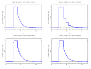
  Optimal relaxed control determined by an indirect approach and by a direct approach on different control discretization grids.

• 

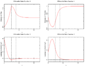
  Differential states and corresponding adjoint variables in the indirect approach.

• 

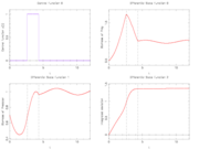
  Control and differential states with only two switches.

• 

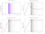
  Control and differential states with 56 switches.

Source Code

Model descriptions are available in

• AMPL code at Lotka Volterra fishing problem (AMPL)
• C code at Lotka Volterra fishing problem (C)
• optimica code at Lotka Volterra fishing problem (optimica)
• JuMP code at Lotka Volterra fishing problem (JuMP)
• Muscod code at Lotka Volterra fishing problem (Muscod)
• ACADO code at Lotka Volterra fishing problem (ACADO)
• VPLAN code at Lotka Volterra fishing problem (VPLAN)
• Casadi code at Lotka Volterra fishing problem (Casadi)
• GloOptCon code at Lotka Volterra fishing problem (GloOptCon)
• switch code at Lotka Volterra fishing problem (switch)

Variants

There are several alternative formulations and variants of the above problem, in particular

• a prescribed time grid for the control function <bibref>Sager2006</bibref>, see also Lotka Volterra fishing problem (AMPL),
• a time-optimal formulation to get into a steady-state <bibref>Sager2005</bibref>,
• the usage of a different target steady-state, as the one corresponding to $w(t) = 1$ which is $(1 + c_1, 1 - c_0)$,
• different fishing control functions for the two species,
• different parameters and start values.

Miscellaneous and Further Reading

The Lotka Volterra fishing problem was introduced by Sebastian Sager in a proceedings paper <bibref>Sager2006</bibref> and revisited in his PhD thesis <bibref>Sager2005</bibref>. These are also the references to look for more details.

References

<bibreferences/>