Difference between revisions of "Lotka Volterra fishing problem"
Henry Chan (Talk | contribs) m (More Knitro testing result by Henry Kar Ming Chan) |
ClemensZeile (Talk | contribs) (→Source Code) |
||
| (40 intermediate revisions by 7 users not shown) | |||
| Line 4: | Line 4: | ||
|nw = 1 | |nw = 1 | ||
|nre = 3 | |nre = 3 | ||
| − | }} | + | }}<!-- Do not insert line break here or Dimensions Box moves up in the layout... |
| − | The '''Lotka Volterra fishing problem''' looks for an optimal fishing strategy to be performed on a fixed time horizon to bring the biomasses of both predator as prey fish to a prescribed steady state. The problem was set up as a small-scale benchmark problem. | + | -->The '''Lotka Volterra fishing problem''' looks for an optimal fishing strategy to be performed on a fixed time horizon to bring the biomasses of both predator as prey fish to a prescribed steady state. The problem was set up as a small-scale benchmark problem. |
The well known [http://en.wikipedia.org/wiki/Lotka_volterra Lotka Volterra equations] for a predator-prey system have been augmented by an additional linear term, relating to fishing by man. The control can be regarded both in a relaxed, as in a discrete manner, corresponding to a part of the fleet, or the full fishing fleet. | The well known [http://en.wikipedia.org/wiki/Lotka_volterra Lotka Volterra equations] for a predator-prey system have been augmented by an additional linear term, relating to fishing by man. The control can be regarded both in a relaxed, as in a discrete manner, corresponding to a part of the fleet, or the full fishing fleet. | ||
| Line 16: | Line 16: | ||
== Mathematical formulation == | == Mathematical formulation == | ||
| − | + | The mixed-integer optimal control problem is given by | |
| + | <p> | ||
<math> | <math> | ||
| − | \begin{array}{ | + | \begin{array}{llclr} |
\displaystyle \min_{x, w} & x_2(t_f) \\[1.5ex] | \displaystyle \min_{x, w} & x_2(t_f) \\[1.5ex] | ||
| − | \mbox{s.t.} & \dot{x}_0 | + | \mbox{s.t.} |
| − | & \dot{x}_1 | + | & \dot{x}_0 & = & x_0 - x_0 x_1 - \; c_0 x_0 \; w, \\ |
| − | & \dot{x}_2 | + | & \dot{x}_1 & = & - x_1 + x_0 x_1 - \; c_1 x_1 \; w, \\ |
| + | & \dot{x}_2 & = & (x_0 - 1)^2 + (x_1 - 1)^2, \\[1.5ex] | ||
& x(0) &=& (0.5, 0.7, 0)^T, \\ | & x(0) &=& (0.5, 0.7, 0)^T, \\ | ||
& w(t) &\in& \{0, 1\}. | & w(t) &\in& \{0, 1\}. | ||
\end{array} | \end{array} | ||
</math> | </math> | ||
| + | </p> | ||
Here the differential states <math>(x_0, x_1)</math> describe the biomasses of prey and predator, respectively. The third differential state is used here to transform the objective, an integrated deviation, into the Mayer formulation <math>\min \; x_2(t_f)</math>. The decision, whether the fishing fleet is actually fishing at time <math>t</math> is denoted by <math>w(t)</math>. | Here the differential states <math>(x_0, x_1)</math> describe the biomasses of prey and predator, respectively. The third differential state is used here to transform the objective, an integrated deviation, into the Mayer formulation <math>\min \; x_2(t_f)</math>. The decision, whether the fishing fleet is actually fishing at time <math>t</math> is denoted by <math>w(t)</math>. | ||
| Line 46: | Line 49: | ||
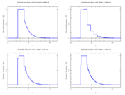
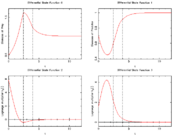
If the problem is relaxed, i.e., we demand that <math>w(t)</math> be in the continuous interval <math>[0, 1]</math> instead of the binary choice <math>\{0,1\}</math>, the optimal solution can be determined by means of [http://en.wikipedia.org/wiki/Pontryagin%27s_minimum_principle Pontryagins maximum principle]. The optimal solution contains a singular arc, as can be seen in the plot of the optimal control. The two differential states and corresponding adjoint variables in the indirect approach are also displayed. A different approach to solving the relaxed problem is by using a direct method such as collocation or Bock's direct multiple shooting method. Optimal solutions for different control discretizations are also plotted in the leftmost figure. | If the problem is relaxed, i.e., we demand that <math>w(t)</math> be in the continuous interval <math>[0, 1]</math> instead of the binary choice <math>\{0,1\}</math>, the optimal solution can be determined by means of [http://en.wikipedia.org/wiki/Pontryagin%27s_minimum_principle Pontryagins maximum principle]. The optimal solution contains a singular arc, as can be seen in the plot of the optimal control. The two differential states and corresponding adjoint variables in the indirect approach are also displayed. A different approach to solving the relaxed problem is by using a direct method such as collocation or Bock's direct multiple shooting method. Optimal solutions for different control discretizations are also plotted in the leftmost figure. | ||
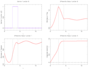
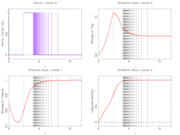
| − | The optimal objective value of this relaxed problem is <math>x_2(t_f) = 1.34408</math>. As follows from MIOC theory< | + | The optimal objective value of this relaxed problem is <math>x_2(t_f) = 1.34408</math>. As follows from MIOC theory <bib id="Sager2011d" /> this is the best lower bound on the optimal value of the original problem with the integer restriction on the control function. In other words, this objective value can be approximated arbitrarily close, if the control only switches often enough between 0 and 1. As no optimal solution exists, two suboptimal ones are shown, one with only two switches and an objective function value of <math>x_2(t_f) = 1.38276</math>, and one with 56 switches and <math>x_2(t_f) = 1.34416</math>. |
<gallery caption="Reference solution plots" widths="180px" heights="140px" perrow="2"> | <gallery caption="Reference solution plots" widths="180px" heights="140px" perrow="2"> | ||
| Line 58: | Line 61: | ||
== Source Code == | == Source Code == | ||
| − | + | Model descriptions are available in | |
| − | + | * [[:Category:ACADO | ACADO code]] at [[Lotka Volterra fishing problem (ACADO)]] | |
| − | + | * [[:Category:AMPL | AMPL code]] at [[Lotka Volterra fishing problem (AMPL)]] | |
| − | + | * [[:Category:APMonitor | APMonitor code]] at [[Lotka Volterra fishing problem (APMonitor)]] | |
| − | + | * [[:Category:Bocop | Bocop code]] at [[Lotka Volterra fishing problem (Bocop)]] | |
| − | + | * [[:Category:Casadi | Casadi code]] at [[Lotka Volterra fishing problem (Casadi)]] | |
| − | + | * [[:Category:Gekko | GEKKO Python code]] at [[Lotka Volterra fishing problem (GEKKO)]] | |
| − | + | * [[:Category:JModelica | JModelica code]] at [[Lotka Volterra fishing problem (JModelica)]] | |
| − | + | * [[:Category:Julia/JuMP | JuMP code]] at [[Lotka Volterra fishing problem (JuMP)]] | |
| − | + | * [[:Category:Muscod | Muscod code]] at [[Lotka Volterra fishing problem (Muscod)]] | |
| − | + | * [[:Category:switch | switch code]] at [[Lotka Volterra fishing problem (switch)]] | |
| − | + | * [[:Category:TomDyn/PROPT | PROPT code]] at [[Lotka Volterra fishing problem (TomDyn/PROPT)]] | |
| − | + | * [[:Category:Julia/JuMP | Julia code]] at [[Lotka Volterra fishing problem (Julia Neural Network solve)]] | |
| − | + | ||
| − | + | ||
| − | + | ||
| − | + | ||
| − | + | ||
| − | + | ||
| − | + | ||
| − | + | ||
| − | + | ||
| − | + | ||
| − | + | ||
| − | + | ||
| − | + | ||
| − | + | ||
| − | + | ||
| − | + | ||
| − | + | ||
| − | + | ||
| − | + | ||
| − | + | ||
| − | + | ||
| − | + | ||
| − | + | ||
| − | + | ||
| − | + | ||
| − | + | ||
| − | + | ||
| − | + | ||
| − | + | ||
| − | + | ||
| − | + | ||
| − | + | ||
| − | + | ||
| − | + | ||
| − | + | ||
| − | + | ||
| − | + | ||
| − | + | ||
| − | + | ||
| − | + | ||
| − | + | ||
| − | + | ||
| − | + | ||
| − | + | ||
| − | + | ||
| − | + | ||
| − | + | ||
| − | + | ||
| − | + | ||
| − | + | ||
| − | + | ||
| − | + | ||
| − | + | ||
| − | + | ||
| − | + | ||
| − | + | ||
| − | + | ||
| − | + | ||
| − | + | ||
| − | + | ||
| − | + | ||
| − | + | ||
| − | + | ||
| − | + | ||
| − | + | ||
| − | + | ||
| − | + | ||
| − | + | ||
| − | + | ||
| − | + | ||
| − | + | ||
| − | + | ||
| − | + | ||
| − | + | ||
| − | + | ||
| − | + | ||
| − | + | ||
| − | + | ||
| − | + | ||
| − | + | ||
| − | + | ||
| − | + | ||
| − | + | ||
| − | + | ||
| − | + | ||
| − | + | ||
| − | + | ||
| − | + | ||
| − | + | ||
| − | + | ||
| − | + | ||
| − | + | ||
| − | + | ||
| − | + | ||
| − | + | ||
| − | * | + | |
| − | + | ||
| − | + | ||
| − | + | ||
| − | + | ||
| − | + | ||
== Variants == | == Variants == | ||
| Line 178: | Line 80: | ||
There are several alternative formulations and variants of the above problem, in particular | There are several alternative formulations and variants of the above problem, in particular | ||
| − | * a prescribed time grid for the control function < | + | * a prescribed time grid for the control function <bib id="Sager2006" />, see also [[Lotka Volterra fishing problem (AMPL)]], |
| − | * a time-optimal formulation to get into a steady-state < | + | * a time-optimal formulation to get into a steady-state <bib id="Sager2005" />, |
| − | * the usage of a different target steady-state, as the one corresponding to <math> w(t) = 1</math> which is <math>(1 + c_1, 1 - c_0)</math>, | + | * the usage of a different target steady-state, as the one corresponding to <math> w(t) = 1</math> which is <math>(1 + c_1, 1 - c_0)</math>, see [[Lotka Volterra multi-arcs problem]] |
| − | * different fishing control functions for the two species, | + | * different fishing control functions for the two species, see [[Lotka Volterra Multimode fishing problem]] |
| + | * different fishing control functions that fish an absolute value from the two species, see [[Lotka Volterra absolute fishing problem]] | ||
| + | * a terminal constrained formulation, where a violation is penalized via slack variables, see [[Lotka Volterra (terminal constraint violation)]] | ||
* different parameters and start values. | * different parameters and start values. | ||
== Miscellaneous and Further Reading == | == Miscellaneous and Further Reading == | ||
| − | The Lotka Volterra fishing problem was introduced by Sebastian Sager in a proceedings paper < | + | The Lotka Volterra fishing problem was introduced by Sebastian Sager in a proceedings paper <bib id="Sager2006" /> and revisited in his PhD thesis <bib id="Sager2005" />. These are also the references to look for more details. |
| − | + | ||
| − | + | ||
| − | + | ||
| − | + | ||
| − | + | ||
| − | + | ||
== References == | == References == | ||
| − | < | + | <biblist /> |
<!--List of all categories this page is part of. List characterization of solution behavior, model properties, ore presence of implementation details (e.g., AMPL for AMPL model) here --> | <!--List of all categories this page is part of. List characterization of solution behavior, model properties, ore presence of implementation details (e.g., AMPL for AMPL model) here --> | ||
| Line 201: | Line 99: | ||
[[Category:Tracking objective]] | [[Category:Tracking objective]] | ||
[[Category:Chattering]] | [[Category:Chattering]] | ||
| − | [[Category: | + | [[Category:Sensitivity-seeking arcs]] |
[[Category:Population dynamics]] | [[Category:Population dynamics]] | ||
| + | |||
| + | |||
| + | <!--Testing Graphviz | ||
| + | <graphviz border='frame' format='svg'> | ||
| + | digraph G {Hello->World!} | ||
| + | </graphviz> | ||
| + | --> | ||
Latest revision as of 17:16, 20 September 2021
| Lotka Volterra fishing problem | |
|---|---|
| State dimension: | 1 |
| Differential states: | 3 |
| Discrete control functions: | 1 |
| Interior point equalities: | 3 |
The Lotka Volterra fishing problem looks for an optimal fishing strategy to be performed on a fixed time horizon to bring the biomasses of both predator as prey fish to a prescribed steady state. The problem was set up as a small-scale benchmark problem. The well known Lotka Volterra equations for a predator-prey system have been augmented by an additional linear term, relating to fishing by man. The control can be regarded both in a relaxed, as in a discrete manner, corresponding to a part of the fleet, or the full fishing fleet.
The mathematical equations form a small-scale ODE model. The interior point equality conditions fix the initial values of the differential states.
The optimal integer control functions shows chattering behavior, making the Lotka Volterra fishing problem an ideal candidate for benchmarking of algorithms.
Contents
[hide]Mathematical formulation
The mixed-integer optimal control problem is given by
![\begin{array}{llclr}
\displaystyle \min_{x, w} & x_2(t_f) \\[1.5ex]
\mbox{s.t.}
& \dot{x}_0 & = & x_0 - x_0 x_1 - \; c_0 x_0 \; w, \\
& \dot{x}_1 & = & - x_1 + x_0 x_1 - \; c_1 x_1 \; w, \\
& \dot{x}_2 & = & (x_0 - 1)^2 + (x_1 - 1)^2, \\[1.5ex]
& x(0) &=& (0.5, 0.7, 0)^T, \\
& w(t) &\in& \{0, 1\}.
\end{array}](https://mintoc.de/images/math/8/1/e/81eae4921b08413ff54a0110dbf48114.png)
Here the differential states  describe the biomasses of prey and predator, respectively. The third differential state is used here to transform the objective, an integrated deviation, into the Mayer formulation
  . The decision, whether the fishing fleet is actually fishing at time
  is denoted by
  .
.
Parameters
These fixed values are used within the model.
![\begin{array}{rcl}
[t_0, t_f] &=& [0, 12],\\
(c_0, c_1) &=& (0.4, 0.2).
\end{array}](https://mintoc.de/images/math/c/0/d/c0d44a47d896216ce3c5ba02b67a90ff.png)
Reference Solutions
If the problem is relaxed, i.e., we demand that  be in the continuous interval
 ![[0, 1]](https://mintoc.de/images/math/c/c/f/ccfcd347d0bf65dc77afe01a3306a96b.png) instead of the binary choice
instead of the binary choice  , the optimal solution can be determined by means of Pontryagins maximum principle. The optimal solution contains a singular arc, as can be seen in the plot of the optimal control. The two differential states and corresponding adjoint variables in the indirect approach are also displayed. A different approach to solving the relaxed problem is by using a direct method such as collocation or Bock's direct multiple shooting method. Optimal solutions for different control discretizations are also plotted in the leftmost figure.
The optimal objective value of this relaxed problem is  . As follows from MIOC theory [Sager2011d]Author: S. Sager
How published: University of Heidelberg
Month: August
Note: Habilitation
Title: On the Integration of Optimization Approaches for Mixed-Integer Nonlinear Optimal Control
Url: http://mathopt.de/PUBLICATIONS/Sager2011d.pdf
Year: 2011 this is the best lower bound on the optimal value of the original problem with the integer restriction on the control function. In other words, this objective value can be approximated arbitrarily close, if the control only switches often enough between 0 and 1. As no optimal solution exists, two suboptimal ones are shown, one with only two switches and an objective function value of
  , and one with 56 switches and
  .
.
- Reference solution plots
Source Code
Model descriptions are available in
- ACADO code at Lotka Volterra fishing problem (ACADO)
- AMPL code at Lotka Volterra fishing problem (AMPL)
- APMonitor code at Lotka Volterra fishing problem (APMonitor)
- Bocop code at Lotka Volterra fishing problem (Bocop)
- Casadi code at Lotka Volterra fishing problem (Casadi)
- GEKKO Python code at Lotka Volterra fishing problem (GEKKO)
- JModelica code at Lotka Volterra fishing problem (JModelica)
- JuMP code at Lotka Volterra fishing problem (JuMP)
- Muscod code at Lotka Volterra fishing problem (Muscod)
- switch code at Lotka Volterra fishing problem (switch)
- PROPT code at Lotka Volterra fishing problem (TomDyn/PROPT)
- Julia code at Lotka Volterra fishing problem (Julia Neural Network solve)
Variants
There are several alternative formulations and variants of the above problem, in particular
- a prescribed time grid for the control function [Sager2006]Address: Heidelberg
Author: S. Sager; H.G. Bock; M. Diehl; G. Reinelt; J.P. Schl\"oder
Booktitle: Recent Advances in Optimization
Editor: A. Seeger
Note: ISBN 978-3-5402-8257-0
Pages: 269--289
Publisher: Springer
Series: Lectures Notes in Economics and Mathematical Systems
Title: Numerical methods for optimal control with binary control functions applied to a Lotka-Volterra type fishing problem
Volume: 563
Year: 2009 , see also Lotka Volterra fishing problem (AMPL),
 - a time-optimal formulation to get into a steady-state [Sager2005]Address: Tönning, Lübeck, Marburg
Author: S. Sager
Editor: ISBN 3-89959-416-9
Publisher: Der andere Verlag
Title: Numerical methods for mixed--integer optimal control problems
Url: http://mathopt.de/PUBLICATIONS/Sager2005.pdf
Year: 2005 ,
, - the usage of a different target steady-state, as the one corresponding to
 which is
  , see Lotka Volterra multi-arcs problem
 - different fishing control functions for the two species, see Lotka Volterra Multimode fishing problem
- different fishing control functions that fish an absolute value from the two species, see Lotka Volterra absolute fishing problem
- a terminal constrained formulation, where a violation is penalized via slack variables, see Lotka Volterra (terminal constraint violation)
- different parameters and start values.
Miscellaneous and Further Reading
The Lotka Volterra fishing problem was introduced by Sebastian Sager in a proceedings paper [Sager2006]Address: Heidelberg
Author: S. Sager; H.G. Bock; M. Diehl; G. Reinelt; J.P. Schl\"oder
Booktitle: Recent Advances in Optimization
Editor: A. Seeger
Note: ISBN 978-3-5402-8257-0
Pages: 269--289
Publisher: Springer
Series: Lectures Notes in Economics and Mathematical Systems
Title: Numerical methods for optimal control with binary control functions applied to a Lotka-Volterra type fishing problem
Volume: 563
Year: 2009 and revisited in his PhD thesis [Sager2005]Address: Tönning, Lübeck, Marburg
Author: S. Sager
Editor: ISBN 3-89959-416-9
Publisher: Der andere Verlag
Title: Numerical methods for mixed--integer optimal control problems
Url: http://mathopt.de/PUBLICATIONS/Sager2005.pdf
Year: 2005 . These are also the references to look for more details.
References
There were no citations found in the article.


